![]()
Basic Fitting with AutoSAS#
This tutorial demonstrates how to use AutoSAS to fit small-angle scattering (SAS) data with different models. We’ll explore how to:
Load and prepare SAS data
Set up an AutoSAS fit for a single model
Compare and evaluate the fits
Google Colab Setup#
Only uncomment and run the next cell if you are running this notebook in Google Colab or if don’t already have the AFL-agent package installed.
[ ]:
# !pip install git+https://github.com/usnistgov/AFL-agent.git
Getting Started#
First, let’s import the necessary packages and load our example dataset:
[5]:
import matplotlib.pyplot as plt

from AFL.double_agent import *
from AFL.double_agent.AutoSAS import AutoSAS
Next, let’s load the example dataset. We’ll subselect only part of the dataset to work with
[6]:
from AFL.double_agent.data import example_dataset2

# Load example dataset and select the mass_fractal model
ds = example_dataset2()
ds = ds.where(ds.model == 'surface_fractal',drop=True)
ds
[6]:
<xarray.Dataset> Size: 17kB
Dimensions:  (sample: 10, q: 100)
Coordinates:
  * q        (q) float64 800B 0.001 0.001072 0.00115 ... 0.8697 0.9326 1.0
Dimensions without coordinates: sample
Data variables:
    I        (sample, q) float64 8kB 5.465e+03 4.598e+03 3.859e+03 ... 1.08 1.03
    dI       (sample, q) float64 8kB 545.9 429.3 342.6 ... 0.1025 0.1025 0.1025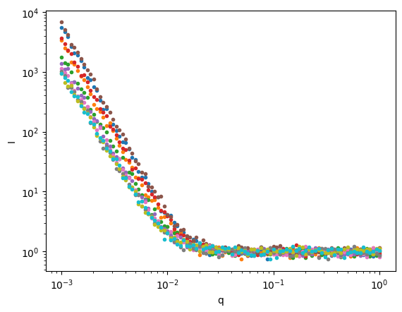
model (sample) object 80B 'surface_fractal' ... 'surface_fractal'Let’s plot the data so we can see what we’re trying to fit.
[7]:
ds.I.plot.line(x='q',xscale='log',yscale='log',marker='.',ls='None',add_legend=False);
Defining the Fit#
The first step to AutoSAS is to define which models we’d like to fit. Let’s start with a single model
The model inputs are defined as a list of dictionaries, where each dictionary specifies:
name: A user-defined name for the modelsasmodel: The name of the model in the sasmodels library to useq_min: the minimum q_value to consider in the fitq_max: the maximum q_value to consider in the fitfit_params: A dictionary of parameters for the model, where:the
valuefield determines the initial starting value for the parameter optimizationthe
boundsfield determines the range that the optimizer can use to fit the data. Restricting this range is very important to achieving a proper fitParameters with “bounds” will be fit within those bounds
Parameters without bounds will be held constant at the specified value
In the example below, “power” and “scale” will be fit since they have bounds, while “background” will be held constant at 1.0
[8]:
model_inputs = [
    {
        "name": "surface_fractal", # your name for the model, can be anything
        "sasmodel": "power_law", # the name of the sasmodel in the sasmodels library
        'q_min':0.001,
        'q_max':1.0,
        "fit_params": {
            "power": {"value": 4, "bounds": (3, 4)},
            "scale": {"value": 1.0, "bounds": (1e-6,1e-3)},
            "background": {"value": 1.0,},
        },
    },
]
Now we’ll create a Pipeline with a single AutoSAS pipeline operation.
The AutoSAS pipeline operation takes several key arguments:
sas_variable: The name of the variable containing the SAS intensity datasas_err_variable: The name of the variable containing the uncertainty in the intensity dataq_dim: The name of the dimension containing the q valuesoutput_prefix: A prefix to add to all output variables from the fitmodel_inputs: A list of dictionaries defining the models to fit, as described above
Additional optional arguments include:
sample_dim: The name of the sample dimension (default: ‘sample’)fit_range: A tuple of (qmin, qmax) to restrict the q range used for fittingmax_evals: Maximum number of function evaluations for the fit (default: 1000)method: The optimization method to use (default: ‘leastsq’)
Building and Executing the Pipeline#
[14]:
with Pipeline() as p:
    AutoSAS(
        sas_variable='I',
        sas_err_variable='dI',
        q_variable = 'q',
        output_prefix='fit',
        model_inputs=model_inputs,
    )
p.print()
PipelineOp                               input_variable ---> output_variable
----------                               -----------------------------------
0  ) <AutoSAS>                           ['q', 'I', 'dI'] ---> ['fit_all_chisq']

Input Variables
---------------
0) q
1) I
2) dI

Output Variables
----------------
0) fit_all_chisq
Now we’re ready to fit!
[15]:
ds_result = p.calculate(ds)
ds_result
[15]:
<xarray.Dataset> Size: 35kB
Dimensions:                    (sample: 10, q: 100, models: 1,
                                surface_fractal_params: 3,
                                fit_q_surface_fractal: 100)
Coordinates:
  * q                          (q) float64 800B 0.001 0.001072 ... 0.9326 1.0
  * models                     (models) <U15 60B 'surface_fractal'
  * surface_fractal_params     (surface_fractal_params) <U26 312B 'surface_fr...
  * fit_q_surface_fractal      (fit_q_surface_fractal) float64 800B 0.001 ......
Dimensions without coordinates: sample
Data variables:
    I                          (sample, q) float64 8kB 5.465e+03 ... 1.03
    dI                         (sample, q) float64 8kB 545.9 429.3 ... 0.1025
    model                      (sample) object 80B 'surface_fractal' ... 'sur...
    sas_fit_sample             (sample) int64 80B 0 1 2 3 4 5 6 7 8 9
    fit_all_chisq              (sample, models) float64 80B 1.023 ... 1.083
    probabilities              (sample, models) float64 80B 1.0 1.0 ... 1.0 1.0
    surface_fractal_fit_val    (surface_fractal_params, sample) float64 240B ...
    surface_fractal_fit_err    (surface_fractal_params, sample) float64 240B ...
    fit_I_surface_fractal      (sample, fit_q_surface_fractal) float64 8kB 5....
residuals_surface_fractal (sample, fit_q_surface_fractal) float64 8kB -0...This is a large and complicated dataset, but it contains all of the information from the fit, including:
The fitted parameter values for each model (e.g.
surface_fractal_fit_val)The uncertainties in the fitted parameters (e.g.
surface_fractal_fit_err)The model intensities at each q value (e.g.
fit_I_surface_fractal)The residuals between the model and data (e.g.
residuals_surface_fractal)The chi-squared values for each fit (
fit_all_chisq)The q values used for the fit (e.g.
fit_q_surface_fractal)
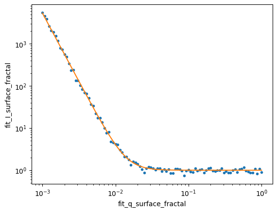
We can use this information to evaluate the quality of the fits and compare different models. Let’s plot some of the fits:
Evaluating the Fit Results#
[16]:
data_index = 0
ds_result.isel(sample=data_index).I.plot.line(x='q',xscale='log',yscale='log',marker='.',ls='None',add_legend=False);
ds_result.isel(sample=data_index).fit_I_surface_fractal.plot.line(x='fit_q_surface_fractal',xscale='log',yscale='log',add_legend=False);
The residuals (differences between the model and data) provide a key way to assess the quality of the fits. A good fit should show residuals that:
Are randomly scattered around zero
Have no clear systematic trends or patterns
Are roughly within ±2-3 standard deviations of zero
Let’s plot the residuals for the first sample to assess the quality of our surface fractal fits:
[17]:
ds_result.isel(sample=data_index).residuals_surface_fractal.plot( x='fit_q_surface_fractal', xscale='log', marker='.', ls='None', add_legend=False)
plt.gca().axhline(y=0, color='k', linestyle='--', alpha=0.5)
[17]:
<matplotlib.lines.Line2D at 0x312294050>
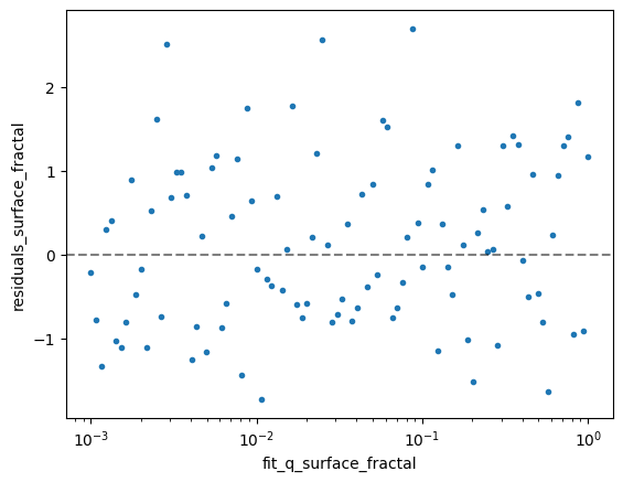
Vary the data_index variable from two cells up and see how well we fit each individual data.
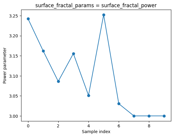
We can also plot the fit parameters
[18]:
# Plot the power parameter (index 1 in surface_fractal_params)
ds_result.sel(surface_fractal_params='surface_fractal_power').surface_fractal_fit_val.plot(marker='o')
plt.ylabel('Power parameter')
plt.xlabel('Sample index')
[18]:
Text(0.5, 0, 'Sample index')
Conclusion#
In this tutorial, we demonstrated how to use the AutoSAS module to fit small-angle scattering (SAS) data. We:
Loaded synthetic dataset with 10 samples and fit it using a surface fractal model
Visualized the fits by plotting the data and model curves on log-log axes
Analyzed the quality of the fits by examining the residuals between the model and data
Explored how the model parameters vary across different samples
The AutoSAS module provides a flexible framework for fitting SAS data with different models, evaluating fit quality, and extracting physical parameters.