![]()
Do Model Selection with AutoSAS#
Google Colab Setup#
Only uncomment and run the next cell if you are running this notebook in Google Colab or if don’t already have the AFL-agent package installed.
[ ]:
# !pip install git+https://github.com/usnistgov/AFL-agent.git
Getting Started#
First, let’s import the necessary packages and load our example dataset:
[1]:
import matplotlib.pyplot as plt

from AFL.double_agent import *
from AFL.double_agent.AutoSAS import AutoSAS
Next, let’s load the example dataset. We’ll subselect only part of the dataset to work with
[2]:
from AFL.double_agent.data import example_dataset2

# Load example dataset and select the mass_fractal model
ds = example_dataset2()
ds = ds.where(ds.model.isin(['surface_fractal','mass_fractal','polymer_excl_volume']),drop=True)
ds
[2]:
<xarray.Dataset> Size: 49kB
Dimensions:  (sample: 30, q: 100)
Coordinates:
  * q        (q) float64 800B 0.001 0.001072 0.00115 ... 0.8697 0.9326 1.0
Dimensions without coordinates: sample
Data variables:
    I        (sample, q) float64 24kB 5.465e+03 4.598e+03 ... 1.1 1.002
    dI       (sample, q) float64 24kB 545.9 429.3 342.6 ... 0.09923 0.09923
model (sample) object 240B 'surface_fractal' ... 'mass_fractal'- sample: 30
- q: 100
- q(q)float640.001 0.001072 ... 0.9326 1.0
array([0.001   , 0.001072, 0.00115 , 0.001233, 0.001322, 0.001417, 0.00152 ,
       0.00163 , 0.001748, 0.001874, 0.002009, 0.002154, 0.00231 , 0.002477,
       0.002656, 0.002848, 0.003054, 0.003275, 0.003511, 0.003765, 0.004037,
       0.004329, 0.004642, 0.004977, 0.005337, 0.005722, 0.006136, 0.006579,
       0.007055, 0.007565, 0.008111, 0.008697, 0.009326, 0.01    , 0.010723,
       0.011498, 0.012328, 0.013219, 0.014175, 0.015199, 0.016298, 0.017475,
       0.018738, 0.020092, 0.021544, 0.023101, 0.024771, 0.026561, 0.02848 ,
       0.030539, 0.032745, 0.035112, 0.037649, 0.04037 , 0.043288, 0.046416,
       0.04977 , 0.053367, 0.057224, 0.061359, 0.065793, 0.070548, 0.075646,
       0.081113, 0.086975, 0.09326 , 0.1     , 0.107227, 0.114976, 0.123285,
       0.132194, 0.141747, 0.151991, 0.162975, 0.174753, 0.187382, 0.200923,
       0.215443, 0.231013, 0.247708, 0.265609, 0.284804, 0.305386, 0.327455,
       0.351119, 0.376494, 0.403702, 0.432876, 0.464159, 0.497702, 0.53367 ,
       0.572237, 0.613591, 0.657933, 0.70548 , 0.756463, 0.811131, 0.869749,
       0.932603, 1.      ])
- I(sample, q)float645.465e+03 4.598e+03 ... 1.1 1.002
array([[5.46461639e+03, 4.59795217e+03, 3.85947764e+03, ..., 8.23637450e-01, 1.08891674e+00, 8.86408253e-01], [1.14146226e+04, 1.20480054e+04, 9.60389049e+03, ..., 1.09249128e+00, 1.03151090e+00, 1.02766190e+00], [3.38673256e+03, 2.48217196e+03, 2.22022900e+03, ..., 1.16251134e+00, 1.01348467e+00, 1.15549165e+00], ..., [2.33984274e+04, 2.43947831e+04, 2.05533255e+04, ..., 1.04267181e+00, 9.85962747e-01, 9.07216458e-01], [2.09634325e+00, 2.08464279e+00, 1.81224765e+00, ..., 1.10735048e+00, 9.92568176e-01, 9.57666868e-01], [1.14052557e+04, 7.68845857e+03, 7.42318078e+03, ..., 1.03875573e+00, 1.10006506e+00, 1.00202285e+00]]) - dI(sample, q)float64545.9 429.3 ... 0.09923 0.09923
array([[5.45853473e+02, 4.29328308e+02, 3.42588723e+02, ..., 9.70709140e-02, 9.70708823e-02, 9.70708568e-02], [1.34833750e+03, 1.10406203e+03, 9.14697444e+02, ..., 1.00109160e-01, 1.00106587e-01, 1.00104428e-01], [3.10385847e+02, 2.45619675e+02, 1.97113531e+02, ..., 9.93385928e-02, 9.93385623e-02, 9.93385376e-02], ..., [2.78764336e+03, 2.26312770e+03, 1.86001084e+03, ..., 9.80268288e-02, 9.80242931e-02, 9.80221832e-02], [2.04875154e-01, 2.04855122e-01, 2.04833121e-01, ..., 1.02022577e-01, 1.02022027e-01, 1.02021575e-01], [1.15537649e+03, 9.47070166e+02, 7.85415799e+02, ..., 9.92344457e-02, 9.92320281e-02, 9.92299984e-02]]) - model(sample)object'surface_fractal' ... 'mass_frac...
array(['surface_fractal', 'mass_fractal', 'surface_fractal',
       'mass_fractal', 'polymer_excl_volume', 'surface_fractal',
       'surface_fractal', 'surface_fractal', 'polymer_excl_volume',
       'mass_fractal', 'mass_fractal', 'polymer_excl_volume',
       'polymer_excl_volume', 'mass_fractal', 'surface_fractal',
       'surface_fractal', 'mass_fractal', 'surface_fractal',
       'surface_fractal', 'surface_fractal', 'polymer_excl_volume',
       'polymer_excl_volume', 'polymer_excl_volume', 'mass_fractal',
       'polymer_excl_volume', 'mass_fractal', 'polymer_excl_volume',
       'mass_fractal', 'polymer_excl_volume', 'mass_fractal'],
      dtype=object)
- qPandasIndex
PandasIndex(Index([                0.001, 0.0010722672220103231, 0.0011497569953977356,
       0.0012328467394420659, 0.0013219411484660286, 0.0014174741629268048,
       0.0015199110829529332, 0.0016297508346206436,  0.001747528400007683,
        0.001873817422860383,  0.002009233002565048, 0.0021544346900318843,
       0.0023101297000831605, 0.0024770763559917113, 0.0026560877829466868,
        0.002848035868435802, 0.0030538555088334154, 0.0032745491628777285,
        0.003511191734215131, 0.0037649358067924675,  0.004037017258596553,
        0.004328761281083057,  0.004641588833612782,  0.004977023564332114,
        0.005336699231206312,   0.00572236765935022,  0.006135907273413176,
        0.006579332246575682,  0.007054802310718645,  0.007564633275546291,
        0.008111308307896872,  0.008697490026177835,    0.0093260334688322,
                        0.01,  0.010722672220103232,  0.011497569953977356,
        0.012328467394420659,  0.013219411484660293,  0.014174741629268055,
         0.01519911082952934,  0.016297508346206444,   0.01747528400007684,
         0.01873817422860384,   0.02009233002565047,  0.021544346900318846,
        0.023101297000831605,  0.024770763559917114,  0.026560877829466867,
         0.02848035868435802,  0.030538555088334154,   0.03274549162877728,
         0.03511191734215131,  0.037649358067924674,   0.04037017258596556,
         0.04328761281083059,  0.046415888336127795,  0.049770235643321115,
          0.0533669923120631,   0.05722367659350217,   0.06135907273413173,
         0.06579332246575682,   0.07054802310718646,   0.07564633275546291,
         0.08111308307896872,   0.08697490026177834,     0.093260334688322,
                         0.1,   0.10722672220103231,   0.11497569953977356,
         0.12328467394420659,   0.13219411484660287,   0.14174741629268048,
          0.1519911082952933,   0.16297508346206452,    0.1747528400007685,
          0.1873817422860385,    0.2009233002565048,   0.21544346900318845,
         0.23101297000831603,   0.24770763559917114,   0.26560877829466867,
          0.2848035868435802,   0.30538555088334157,   0.32745491628777285,
          0.3511191734215131,   0.37649358067924676,   0.40370172585965536,
          0.4328761281083057,    0.4641588833612782,   0.49770235643321137,
          0.5336699231206312,     0.572236765935022,    0.6135907273413176,
          0.6579332246575682,    0.7054802310718645,    0.7564633275546291,
          0.8111308307896873,    0.8697490026177834,    0.9326033468832199,
                         1.0],
      dtype='float64', name='q'))
Let’s plot the data so we can see what we’re trying to fit.
[3]:
for model,sds in ds.groupby('model'):
    plt.figure()
    sds.I.plot.line(x='q',xscale='log',yscale='log',marker='.',ls='None',add_legend=False);
    plt.title(model)

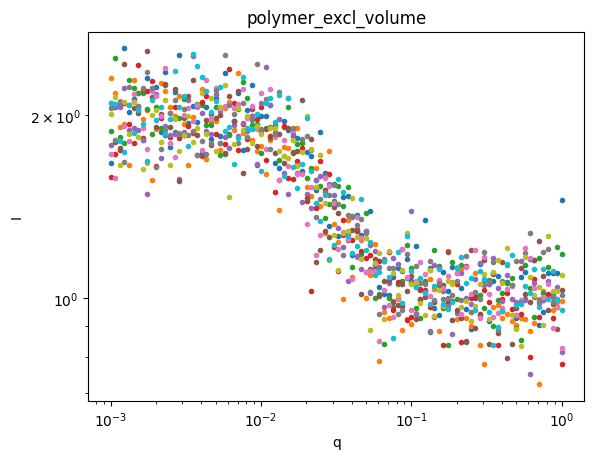
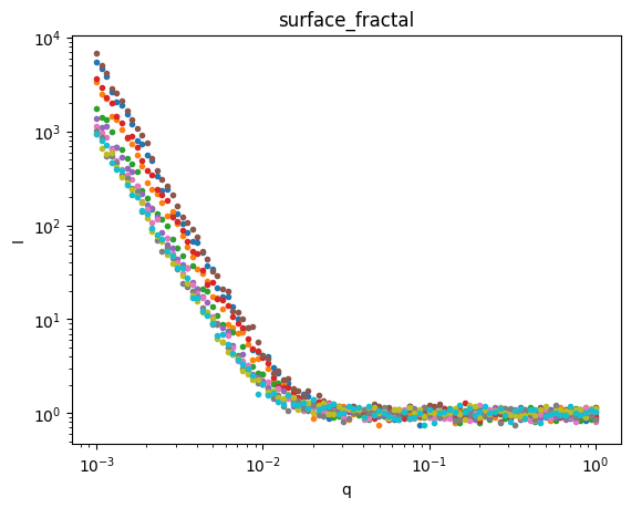
Great, we have three groups of data. Let’s use AutoSAS to fit and classify this data.
Defining the Fit#
The first step to AutoSAS is to define which models we’d like to fit. Since we have three representations of data in our dataset, we’ll define three models to fit it. In real, experimental scenarios, you often don’t know how many structures you might encounter, so you can define as many as you’d like in the model_input list.
[20]:
model_inputs = [
    {
        "name": "surface_fractal", # your name for the model, can be anything
        "sasmodel": "power_law", # the name of the sasmodel in the sasmodels library
        'q_min':0.001,
        'q_max':1.0,
        "fit_params": {
            "power": {"value": 4, "bounds": (3, 4)},
            "scale": {"value": 1.0, "bounds": (1e-6,1e-3)},
            "background": {"value": 1.0},
        },
    },
    {
        "name": "mass_fractal",
        "sasmodel": "power_law",
        'q_min':0.001,
        'q_max':1.0,
        "fit_params": {
            "power": {"value": 4, "bounds": (1.7, 3)},
            "scale": {"value": 1.0, "bounds": (1e-4,1e-1)},
            "background": {"value": 1.0},
        },
    },
    {
        "name": "polymer",
        "sasmodel": "polymer_excl_volume",
        'q_min':0.001,
        'q_max':1.0,
        "fit_params": {
            "scale": {"value": 1.0, "bounds": (1e-2,1e2)},
            "rg": {"value": 60.0, "bounds": (10,150)},
            "background": {"value": 1.0},
        },
    }
]
Building and Executing the Pipeline#
We then construct a pipeline with a single pipeline operation. We tell the operation what the data will be named in the dataset and give it the list of model inputs.
[43]:
with Pipeline() as autosas_pipeline1:
    AutoSAS(
        sas_variable='I',
        sas_err_variable='dI',
        q_variable = 'q',
        output_prefix='fit',
        model_inputs=model_inputs,
    )
autosas_pipeline1.print()
PipelineOp                               input_variable ---> output_variable
----------                               -----------------------------------
0  ) <AutoSAS>                           ['q', 'I', 'dI'] ---> ['fit_all_chisq']

Input Variables
---------------
0) q
1) I
2) dI

Output Variables
----------------
0) fit_all_chisq
Now we’re ready to fit! When we run the pipeline, it will fit each of the three models in model_input to every measurement in the dataset. For this dataset, that means that we’ll carry out 90 fits.
[ ]:
ds_result = autosas_pipeline1.calculate(ds)
ds_result
<xarray.Dataset> Size: 202kB
Dimensions:                    (sample: 30, q: 100, models: 3,
                                surface_fractal_params: 3,
                                mass_fractal_params: 3, polymer_params: 3,
                                fit_q_surface_fractal: 100,
                                fit_q_mass_fractal: 100, fit_q_polymer: 100)
Coordinates:
  * q                          (q) float64 800B 0.001 0.001072 ... 0.9326 1.0
  * models                     (models) <U15 180B 'surface_fractal' ... 'poly...
  * surface_fractal_params     (surface_fractal_params) <U26 312B 'surface_fr...
  * mass_fractal_params        (mass_fractal_params) <U23 276B 'mass_fractal_...
  * polymer_params             (polymer_params) <U18 216B 'polymer_scale' ......
  * fit_q_surface_fractal      (fit_q_surface_fractal) float64 800B 0.001 ......
  * fit_q_mass_fractal         (fit_q_mass_fractal) float64 800B 0.001 ... 1.0
  * fit_q_polymer              (fit_q_polymer) float64 800B 0.001 ... 1.0
Dimensions without coordinates: sample
Data variables: (12/18)
    I                          (sample, q) float64 24kB 5.465e+03 ... 1.002
    dI                         (sample, q) float64 24kB 545.9 429.3 ... 0.09923
    model                      (sample) object 240B 'surface_fractal' ... 'ma...
    sas_fit_sample             (sample) int64 240B 0 1 2 3 4 ... 25 26 27 28 29
    fit_all_chisq              (sample, models) float64 720B 1.023 ... 27.2
    probabilities              (sample, models) float64 720B 0.01182 ... 0.00...
    ...                         ...
    fit_I_surface_fractal      (sample, fit_q_surface_fractal) float64 24kB 5...
    residuals_surface_fractal  (sample, fit_q_surface_fractal) float64 24kB -...
    fit_I_mass_fractal         (sample, fit_q_mass_fractal) float64 24kB 956....
    residuals_mass_fractal     (sample, fit_q_mass_fractal) float64 24kB -8.2...
    fit_I_polymer              (sample, fit_q_polymer) float64 24kB 6.219 ......
residuals_polymer (sample, fit_q_polymer) float64 24kB -10.0 ......- sample: 30
- q: 100
- models: 3
- surface_fractal_params: 3
- mass_fractal_params: 3
- polymer_params: 3
- fit_q_surface_fractal: 100
- fit_q_mass_fractal: 100
- fit_q_polymer: 100
- q(q)float640.001 0.001072 ... 0.9326 1.0
array([0.001 , 0.001072, 0.00115 , 0.001233, 0.001322, 0.001417, 0.00152 , 0.00163 , 0.001748, 0.001874, 0.002009, 0.002154, 0.00231 , 0.002477, 0.002656, 0.002848, 0.003054, 0.003275, 0.003511, 0.003765, 0.004037, 0.004329, 0.004642, 0.004977, 0.005337, 0.005722, 0.006136, 0.006579, 0.007055, 0.007565, 0.008111, 0.008697, 0.009326, 0.01 , 0.010723, 0.011498, 0.012328, 0.013219, 0.014175, 0.015199, 0.016298, 0.017475, 0.018738, 0.020092, 0.021544, 0.023101, 0.024771, 0.026561, 0.02848 , 0.030539, 0.032745, 0.035112, 0.037649, 0.04037 , 0.043288, 0.046416, 0.04977 , 0.053367, 0.057224, 0.061359, 0.065793, 0.070548, 0.075646, 0.081113, 0.086975, 0.09326 , 0.1 , 0.107227, 0.114976, 0.123285, 0.132194, 0.141747, 0.151991, 0.162975, 0.174753, 0.187382, 0.200923, 0.215443, 0.231013, 0.247708, 0.265609, 0.284804, 0.305386, 0.327455, 0.351119, 0.376494, 0.403702, 0.432876, 0.464159, 0.497702, 0.53367 , 0.572237, 0.613591, 0.657933, 0.70548 , 0.756463, 0.811131, 0.869749, 0.932603, 1. ]) - models(models)<U15'surface_fractal' ... 'polymer'
array(['surface_fractal', 'mass_fractal', 'polymer'], dtype='<U15')
- surface_fractal_params(surface_fractal_params)<U26'surface_fractal_power' ... 'sur...
array(['surface_fractal_power', 'surface_fractal_scale', 'surface_fractal_background'], dtype='<U26') - mass_fractal_params(mass_fractal_params)<U23'mass_fractal_power' ... 'mass_f...
array(['mass_fractal_power', 'mass_fractal_scale', 'mass_fractal_background'], dtype='<U23') - polymer_params(polymer_params)<U18'polymer_scale' ... 'polymer_bac...
array(['polymer_scale', 'polymer_rg', 'polymer_background'], dtype='<U18')
- fit_q_surface_fractal(fit_q_surface_fractal)float640.001 0.001072 ... 0.9326 1.0
array([0.001 , 0.001072, 0.00115 , 0.001233, 0.001322, 0.001417, 0.00152 , 0.00163 , 0.001748, 0.001874, 0.002009, 0.002154, 0.00231 , 0.002477, 0.002656, 0.002848, 0.003054, 0.003275, 0.003511, 0.003765, 0.004037, 0.004329, 0.004642, 0.004977, 0.005337, 0.005722, 0.006136, 0.006579, 0.007055, 0.007565, 0.008111, 0.008697, 0.009326, 0.01 , 0.010723, 0.011498, 0.012328, 0.013219, 0.014175, 0.015199, 0.016298, 0.017475, 0.018738, 0.020092, 0.021544, 0.023101, 0.024771, 0.026561, 0.02848 , 0.030539, 0.032745, 0.035112, 0.037649, 0.04037 , 0.043288, 0.046416, 0.04977 , 0.053367, 0.057224, 0.061359, 0.065793, 0.070548, 0.075646, 0.081113, 0.086975, 0.09326 , 0.1 , 0.107227, 0.114976, 0.123285, 0.132194, 0.141747, 0.151991, 0.162975, 0.174753, 0.187382, 0.200923, 0.215443, 0.231013, 0.247708, 0.265609, 0.284804, 0.305386, 0.327455, 0.351119, 0.376494, 0.403702, 0.432876, 0.464159, 0.497702, 0.53367 , 0.572237, 0.613591, 0.657933, 0.70548 , 0.756463, 0.811131, 0.869749, 0.932603, 1. ]) - fit_q_mass_fractal(fit_q_mass_fractal)float640.001 0.001072 ... 0.9326 1.0
array([0.001 , 0.001072, 0.00115 , 0.001233, 0.001322, 0.001417, 0.00152 , 0.00163 , 0.001748, 0.001874, 0.002009, 0.002154, 0.00231 , 0.002477, 0.002656, 0.002848, 0.003054, 0.003275, 0.003511, 0.003765, 0.004037, 0.004329, 0.004642, 0.004977, 0.005337, 0.005722, 0.006136, 0.006579, 0.007055, 0.007565, 0.008111, 0.008697, 0.009326, 0.01 , 0.010723, 0.011498, 0.012328, 0.013219, 0.014175, 0.015199, 0.016298, 0.017475, 0.018738, 0.020092, 0.021544, 0.023101, 0.024771, 0.026561, 0.02848 , 0.030539, 0.032745, 0.035112, 0.037649, 0.04037 , 0.043288, 0.046416, 0.04977 , 0.053367, 0.057224, 0.061359, 0.065793, 0.070548, 0.075646, 0.081113, 0.086975, 0.09326 , 0.1 , 0.107227, 0.114976, 0.123285, 0.132194, 0.141747, 0.151991, 0.162975, 0.174753, 0.187382, 0.200923, 0.215443, 0.231013, 0.247708, 0.265609, 0.284804, 0.305386, 0.327455, 0.351119, 0.376494, 0.403702, 0.432876, 0.464159, 0.497702, 0.53367 , 0.572237, 0.613591, 0.657933, 0.70548 , 0.756463, 0.811131, 0.869749, 0.932603, 1. ]) - fit_q_polymer(fit_q_polymer)float640.001 0.001072 ... 0.9326 1.0
array([0.001   , 0.001072, 0.00115 , 0.001233, 0.001322, 0.001417, 0.00152 ,
       0.00163 , 0.001748, 0.001874, 0.002009, 0.002154, 0.00231 , 0.002477,
       0.002656, 0.002848, 0.003054, 0.003275, 0.003511, 0.003765, 0.004037,
       0.004329, 0.004642, 0.004977, 0.005337, 0.005722, 0.006136, 0.006579,
       0.007055, 0.007565, 0.008111, 0.008697, 0.009326, 0.01    , 0.010723,
       0.011498, 0.012328, 0.013219, 0.014175, 0.015199, 0.016298, 0.017475,
       0.018738, 0.020092, 0.021544, 0.023101, 0.024771, 0.026561, 0.02848 ,
       0.030539, 0.032745, 0.035112, 0.037649, 0.04037 , 0.043288, 0.046416,
       0.04977 , 0.053367, 0.057224, 0.061359, 0.065793, 0.070548, 0.075646,
       0.081113, 0.086975, 0.09326 , 0.1     , 0.107227, 0.114976, 0.123285,
       0.132194, 0.141747, 0.151991, 0.162975, 0.174753, 0.187382, 0.200923,
       0.215443, 0.231013, 0.247708, 0.265609, 0.284804, 0.305386, 0.327455,
       0.351119, 0.376494, 0.403702, 0.432876, 0.464159, 0.497702, 0.53367 ,
       0.572237, 0.613591, 0.657933, 0.70548 , 0.756463, 0.811131, 0.869749,
       0.932603, 1.      ])
- I(sample, q)float645.465e+03 4.598e+03 ... 1.1 1.002
array([[5.46461639e+03, 4.59795217e+03, 3.85947764e+03, ..., 8.23637450e-01, 1.08891674e+00, 8.86408253e-01], [1.14146226e+04, 1.20480054e+04, 9.60389049e+03, ..., 1.09249128e+00, 1.03151090e+00, 1.02766190e+00], [3.38673256e+03, 2.48217196e+03, 2.22022900e+03, ..., 1.16251134e+00, 1.01348467e+00, 1.15549165e+00], ..., [2.33984274e+04, 2.43947831e+04, 2.05533255e+04, ..., 1.04267181e+00, 9.85962747e-01, 9.07216458e-01], [2.09634325e+00, 2.08464279e+00, 1.81224765e+00, ..., 1.10735048e+00, 9.92568176e-01, 9.57666868e-01], [1.14052557e+04, 7.68845857e+03, 7.42318078e+03, ..., 1.03875573e+00, 1.10006506e+00, 1.00202285e+00]]) - dI(sample, q)float64545.9 429.3 ... 0.09923 0.09923
array([[5.45853473e+02, 4.29328308e+02, 3.42588723e+02, ..., 9.70709140e-02, 9.70708823e-02, 9.70708568e-02], [1.34833750e+03, 1.10406203e+03, 9.14697444e+02, ..., 1.00109160e-01, 1.00106587e-01, 1.00104428e-01], [3.10385847e+02, 2.45619675e+02, 1.97113531e+02, ..., 9.93385928e-02, 9.93385623e-02, 9.93385376e-02], ..., [2.78764336e+03, 2.26312770e+03, 1.86001084e+03, ..., 9.80268288e-02, 9.80242931e-02, 9.80221832e-02], [2.04875154e-01, 2.04855122e-01, 2.04833121e-01, ..., 1.02022577e-01, 1.02022027e-01, 1.02021575e-01], [1.15537649e+03, 9.47070166e+02, 7.85415799e+02, ..., 9.92344457e-02, 9.92320281e-02, 9.92299984e-02]]) - model(sample)object'surface_fractal' ... 'mass_frac...
array(['surface_fractal', 'mass_fractal', 'surface_fractal', 'mass_fractal', 'polymer_excl_volume', 'surface_fractal', 'surface_fractal', 'surface_fractal', 'polymer_excl_volume', 'mass_fractal', 'mass_fractal', 'polymer_excl_volume', 'polymer_excl_volume', 'mass_fractal', 'surface_fractal', 'surface_fractal', 'mass_fractal', 'surface_fractal', 'surface_fractal', 'surface_fractal', 'polymer_excl_volume', 'polymer_excl_volume', 'polymer_excl_volume', 'mass_fractal', 'polymer_excl_volume', 'mass_fractal', 'polymer_excl_volume', 'mass_fractal', 'polymer_excl_volume', 'mass_fractal'], dtype=object) - sas_fit_sample(sample)int640 1 2 3 4 5 6 ... 24 25 26 27 28 29
- name :
- AutoSAS
- input_variable :
- ['q', 'I', 'dI']
- output_variable :
- ['fit_all_chisq']
- input_prefix :
- None
- output_prefix :
- fit
- server_id :
- None
- fit_method :
- None
- model_inputs :
- [{'name': 'surface_fractal', 'sasmodel': 'power_law', 'q_min': 0.001, 'q_max': 1.0, 'fit_params': {'power': {'value': 4, 'bounds': (3, 4)}, 'scale': {'value': 1.0, 'bounds': (1e-06, 0.001)}, 'background': {'value': 1.0}}}, {'name': 'mass_fractal', 'sasmodel': 'power_law', 'q_min': 0.001, 'q_max': 1.0, 'fit_params': {'power': {'value': 4, 'bounds': (1.7, 3)}, 'scale': {'value': 1.0, 'bounds': (0.0001, 0.1)}, 'background': {'value': 1.0}}}, {'name': 'polymer', 'sasmodel': 'polymer_excl_volume', 'q_min': 0.001, 'q_max': 1.0, 'fit_params': {'scale': {'value': 1.0, 'bounds': (0.01, 100.0)}, 'rg': {'value': 60.0, 'bounds': (10, 150)}, 'background': {'value': 1.0}}}]
- results :
- {}
- q_variable :
- q
- sas_variable :
- I
- sas_err_variable :
- dI
- resolution :
- None
- sample_dim :
- sample
- model_dim :
- models
- q_min :
- None
- q_max :
- None
array([ 0, 1, 2, 3, 4, 5, 6, 7, 8, 9, 10, 11, 12, 13, 14, 15, 16, 17, 18, 19, 20, 21, 22, 23, 24, 25, 26, 27, 28, 29]) - fit_all_chisq(sample, models)float641.023 14.07 27.32 ... 1.086 27.2
- fit_calc_id :
- ASAS-a69b1c5c-c1d3-4c5e-a758-0fc3f5c1525e
- name :
- AutoSAS
- input_variable :
- ['q', 'I', 'dI']
- output_variable :
- ['fit_all_chisq']
- input_prefix :
- None
- output_prefix :
- fit
- server_id :
- None
- fit_method :
- None
- model_inputs :
- [{'name': 'surface_fractal', 'sasmodel': 'power_law', 'q_min': 0.001, 'q_max': 1.0, 'fit_params': {'power': {'value': 4, 'bounds': (3, 4)}, 'scale': {'value': 1.0, 'bounds': (1e-06, 0.001)}, 'background': {'value': 1.0}}}, {'name': 'mass_fractal', 'sasmodel': 'power_law', 'q_min': 0.001, 'q_max': 1.0, 'fit_params': {'power': {'value': 4, 'bounds': (1.7, 3)}, 'scale': {'value': 1.0, 'bounds': (0.0001, 0.1)}, 'background': {'value': 1.0}}}, {'name': 'polymer', 'sasmodel': 'polymer_excl_volume', 'q_min': 0.001, 'q_max': 1.0, 'fit_params': {'scale': {'value': 1.0, 'bounds': (0.01, 100.0)}, 'rg': {'value': 60.0, 'bounds': (10, 150)}, 'background': {'value': 1.0}}}]
- results :
- {}
- q_variable :
- q
- sas_variable :
- I
- sas_err_variable :
- dI
- resolution :
- None
- sample_dim :
- sample
- model_dim :
- models
- q_min :
- None
- q_max :
- None
array([[1.02275423e+00, 1.40722782e+01, 2.73224420e+01], [4.09722407e+00, 9.50171680e-01, 2.63673388e+01], [1.05413472e+00, 1.36841369e+01, 2.72866689e+01], [1.14629265e+00, 1.04990624e+00, 3.17019675e+01], [6.96376204e+05, 1.35878440e+02, 1.18324132e+00], [1.08126923e+00, 1.19570931e+01, 2.58392185e+01], [8.36611432e-01, 1.21540498e+01, 2.69767485e+01], [8.92581487e-01, 1.12844843e+01, 2.53700558e+01], [7.43408306e+05, 1.44644370e+02, 1.11691133e+00], [4.08984295e+00, 9.12932757e-01, 2.64968640e+01], [1.32050220e+00, 9.75581038e-01, 3.07720967e+01], [7.06812364e+05, 1.37343734e+02, 9.18066715e-01], [7.71372671e+05, 1.56599393e+02, 9.73842068e-01], [1.57930523e+00, 1.01924014e+00, 3.04306793e+01], [9.31217832e-01, 1.24766894e+01, 2.55126991e+01], [9.27394330e-01, 1.03076313e+01, 2.44011743e+01], [4.01568675e+00, 8.51332910e-01, 2.83843343e+01], [1.07638344e+00, 1.05327569e+01, 2.38169213e+01], [8.71404947e-01, 8.93694309e+00, 2.19797127e+01], [1.08324978e+00, 9.81511077e+00, 2.41165279e+01], [7.36691528e+05, 1.47836036e+02, 1.09358942e+00], [7.15150775e+05, 1.38734930e+02, 1.10718714e+00], [7.28863488e+05, 1.47481645e+02, 9.61265988e-01], [2.05590837e+00, 1.13113537e+00, 2.80256684e+01], [7.30479177e+05, 1.44870136e+02, 1.03919799e+00], [1.23729309e+00, 8.66385752e-01, 2.81719466e+01], [7.49889915e+05, 1.51181543e+02, 9.99128955e-01], [2.42291207e+00, 1.16555890e+00, 3.01412948e+01], [7.08550329e+05, 1.41412767e+02, 1.08373657e+00], [4.75962943e+00, 1.08625395e+00, 2.72039930e+01]]) - probabilities(sample, models)float640.01182 0.9238 ... 0.9984 0.001121
- name :
- AutoSAS
- input_variable :
- ['q', 'I', 'dI']
- output_variable :
- ['fit_all_chisq']
- input_prefix :
- None
- output_prefix :
- fit
- server_id :
- None
- fit_method :
- None
- model_inputs :
- [{'name': 'surface_fractal', 'sasmodel': 'power_law', 'q_min': 0.001, 'q_max': 1.0, 'fit_params': {'power': {'value': 4, 'bounds': (3, 4)}, 'scale': {'value': 1.0, 'bounds': (1e-06, 0.001)}, 'background': {'value': 1.0}}}, {'name': 'mass_fractal', 'sasmodel': 'power_law', 'q_min': 0.001, 'q_max': 1.0, 'fit_params': {'power': {'value': 4, 'bounds': (1.7, 3)}, 'scale': {'value': 1.0, 'bounds': (0.0001, 0.1)}, 'background': {'value': 1.0}}}, {'name': 'polymer', 'sasmodel': 'polymer_excl_volume', 'q_min': 0.001, 'q_max': 1.0, 'fit_params': {'scale': {'value': 1.0, 'bounds': (0.01, 100.0)}, 'rg': {'value': 60.0, 'bounds': (10, 150)}, 'background': {'value': 1.0}}}]
- results :
- {}
- q_variable :
- q
- sas_variable :
- I
- sas_err_variable :
- dI
- resolution :
- None
- sample_dim :
- sample
- model_dim :
- models
- q_min :
- None
- q_max :
- None
array([[1.18241649e-02, 9.23820654e-01, 6.43551809e-02], [1.23607135e-03, 9.96341125e-01, 2.42280337e-03], [8.23266617e-03, 9.40641961e-01, 5.11253726e-02], [4.27533439e-01, 5.72377505e-01, 8.90553923e-05], [0.00000000e+00, 1.73073808e-64, 1.00000000e+00], [1.49740488e-03, 9.57828584e-01, 4.06740111e-02], [3.55950627e-03, 9.80632154e-01, 1.58083397e-02], [9.17293426e-04, 9.47240896e-01, 5.18418105e-02], [0.00000000e+00, 1.78346827e-68, 1.00000000e+00], [1.27297309e-02, 9.85285111e-01, 1.98515819e-03], [3.07295385e-01, 6.92659281e-01, 4.53336987e-05], [0.00000000e+00, 2.87852843e-65, 1.00000000e+00], [0.00000000e+00, 9.22602333e-74, 1.00000000e+00], [2.61966631e-01, 7.37981212e-01, 5.21571954e-05], [3.16094856e-03, 9.03018069e-01, 9.38209827e-02], [3.49580420e-04, 9.71200269e-01, 2.84501501e-02], [1.29078990e-02, 9.86763088e-01, 3.29012466e-04], [3.03155123e-04, 7.98369591e-01, 2.01327254e-01], [8.19662930e-05, 9.22293393e-01, 7.76246408e-02], [1.01633723e-04, 5.47733346e-01, 4.52165021e-01], [0.00000000e+00, 7.95457604e-70, 1.00000000e+00], [0.00000000e+00, 6.45880860e-66, 1.00000000e+00], [0.00000000e+00, 8.57179161e-70, 1.00000000e+00], [1.74573275e-01, 8.24542384e-01, 8.84340955e-04], [0.00000000e+00, 1.81958266e-68, 1.00000000e+00], [3.19004059e-01, 6.80291474e-01, 7.04467341e-04], [0.00000000e+00, 2.68265729e-71, 1.00000000e+00], [1.02787938e-01, 8.97121386e-01, 9.06757543e-05], [0.00000000e+00, 5.10032208e-67, 1.00000000e+00], [5.20020767e-04, 9.98358893e-01, 1.12108653e-03]]) - surface_fractal_fit_val(surface_fractal_params, sample)float643.243 3.0 3.163 3.0 ... 1.0 1.0 1.0
- fit_calc_id :
- ASAS-a69b1c5c-c1d3-4c5e-a758-0fc3f5c1525e
- name :
- AutoSAS
- input_variable :
- ['q', 'I', 'dI']
- output_variable :
- ['fit_all_chisq']
- input_prefix :
- None
- output_prefix :
- fit
- server_id :
- None
- fit_method :
- None
- model_inputs :
- [{'name': 'surface_fractal', 'sasmodel': 'power_law', 'q_min': 0.001, 'q_max': 1.0, 'fit_params': {'power': {'value': 4, 'bounds': (3, 4)}, 'scale': {'value': 1.0, 'bounds': (1e-06, 0.001)}, 'background': {'value': 1.0}}}, {'name': 'mass_fractal', 'sasmodel': 'power_law', 'q_min': 0.001, 'q_max': 1.0, 'fit_params': {'power': {'value': 4, 'bounds': (1.7, 3)}, 'scale': {'value': 1.0, 'bounds': (0.0001, 0.1)}, 'background': {'value': 1.0}}}, {'name': 'polymer', 'sasmodel': 'polymer_excl_volume', 'q_min': 0.001, 'q_max': 1.0, 'fit_params': {'scale': {'value': 1.0, 'bounds': (0.01, 100.0)}, 'rg': {'value': 60.0, 'bounds': (10, 150)}, 'background': {'value': 1.0}}}]
- results :
- {}
- q_variable :
- q
- sas_variable :
- I
- sas_err_variable :
- dI
- resolution :
- None
- sample_dim :
- sample
- model_dim :
- models
- q_min :
- None
- q_max :
- None
array([[3.24265739e+00, 3.00000000e+00, 3.16252070e+00, 3.00000000e+00, 3.00000000e+00, 3.08615609e+00, 3.15552503e+00, 3.05113167e+00, 3.00000000e+00, 3.00000000e+00, 3.00000000e+00, 3.00000000e+00, 3.00000000e+00, 3.00000000e+00, 3.25242366e+00, 3.03037286e+00, 3.00000000e+00, 3.00000000e+00, 3.00000000e+00, 3.00000000e+00, 3.00000000e+00, 3.00000000e+00, 3.00000000e+00, 3.00000000e+00, 3.00000000e+00, 3.00000000e+00, 3.00000000e+00, 3.00000000e+00, 3.00000000e+00, 3.00000000e+00], [1.00000000e-06, 1.88805902e-05, 1.00000000e-06, 8.07491165e-05, 1.00000000e-06, 1.00000000e-06, 1.24393004e-06, 1.00000000e-06, 1.00000000e-06, 2.18202275e-05, 6.10328588e-05, 1.00000000e-06, 1.00000000e-06, 5.96185299e-05, 1.11492212e-06, 1.00000000e-06, 2.25881511e-05, 1.00000000e-06, 1.00000000e-06, 1.00000000e-06, 1.00000000e-06, 1.00000000e-06, 1.00000000e-06, 5.01149203e-05, 1.00000000e-06, 6.92824955e-05, 1.00000000e-06, 3.59572491e-05, 1.00000000e-06, 1.64517485e-05], [1.00000000e+00, 1.00000000e+00, 1.00000000e+00, 1.00000000e+00, 1.00000000e+00, 1.00000000e+00, 1.00000000e+00, 1.00000000e+00, 1.00000000e+00, 1.00000000e+00, 1.00000000e+00, 1.00000000e+00, 1.00000000e+00, 1.00000000e+00, 1.00000000e+00, 1.00000000e+00, 1.00000000e+00, 1.00000000e+00, 1.00000000e+00, 1.00000000e+00, 1.00000000e+00, 1.00000000e+00, 1.00000000e+00, 1.00000000e+00, 1.00000000e+00, 1.00000000e+00, 1.00000000e+00, 1.00000000e+00, 1.00000000e+00, 1.00000000e+00]]) - surface_fractal_fit_err(surface_fractal_params, sample)float640.0227 0.01792 0.02407 ... 0.0 0.0
- fit_calc_id :
- ASAS-a69b1c5c-c1d3-4c5e-a758-0fc3f5c1525e
- name :
- AutoSAS
- input_variable :
- ['q', 'I', 'dI']
- output_variable :
- ['fit_all_chisq']
- input_prefix :
- None
- output_prefix :
- fit
- server_id :
- None
- fit_method :
- None
- model_inputs :
- [{'name': 'surface_fractal', 'sasmodel': 'power_law', 'q_min': 0.001, 'q_max': 1.0, 'fit_params': {'power': {'value': 4, 'bounds': (3, 4)}, 'scale': {'value': 1.0, 'bounds': (1e-06, 0.001)}, 'background': {'value': 1.0}}}, {'name': 'mass_fractal', 'sasmodel': 'power_law', 'q_min': 0.001, 'q_max': 1.0, 'fit_params': {'power': {'value': 4, 'bounds': (1.7, 3)}, 'scale': {'value': 1.0, 'bounds': (0.0001, 0.1)}, 'background': {'value': 1.0}}}, {'name': 'polymer', 'sasmodel': 'polymer_excl_volume', 'q_min': 0.001, 'q_max': 1.0, 'fit_params': {'scale': {'value': 1.0, 'bounds': (0.01, 100.0)}, 'rg': {'value': 60.0, 'bounds': (10, 150)}, 'background': {'value': 1.0}}}]
- results :
- {}
- q_variable :
- q
- sas_variable :
- I
- sas_err_variable :
- dI
- resolution :
- None
- sample_dim :
- sample
- model_dim :
- models
- q_min :
- None
- q_max :
- None
array([[2.27048704e-02, 1.79223126e-02, 2.40659471e-02, 1.30755205e-02, 7.27887423e-04, 2.55743991e-02, 2.29994739e-02, 2.63328387e-02, 7.04419584e-04, 1.73100251e-02, 1.37324240e-02, 7.22326241e-04, 6.91839641e-04, 1.39774626e-02, 2.28313482e-02, 2.70634988e-02, 1.68284235e-02, 2.78456852e-02, 2.78247365e-02, 2.77249316e-02, 7.07711080e-04, 7.18157333e-04, 7.11603537e-04, 1.46252174e-02, 7.10825868e-04, 1.38115165e-02, 7.01610295e-04, 1.51664322e-02, 7.21627230e-04, 1.82691043e-02], [1.30712675e-07, 1.99407460e-06, 1.39863344e-07, 5.68296258e-06, 4.93677731e-09, 1.49719861e-07, 1.64556199e-07, 1.55220020e-07, 4.77760508e-09, 2.21210410e-06, 4.59230273e-06, 4.89904463e-09, 4.69228908e-09, 4.58996792e-06, 1.45467891e-07, 1.59749280e-07, 2.22355435e-06, 1.64812550e-07, 1.64903795e-07, 1.64396226e-07, 4.79992379e-09, 4.87077236e-09, 4.82632551e-09, 4.07911051e-06, 4.82106811e-09, 5.20163539e-06, 4.75856119e-09, 3.10007783e-06, 4.89431125e-09, 1.77906351e-06], [0.00000000e+00, 0.00000000e+00, 0.00000000e+00, 0.00000000e+00, 0.00000000e+00, 0.00000000e+00, 0.00000000e+00, 0.00000000e+00, 0.00000000e+00, 0.00000000e+00, 0.00000000e+00, 0.00000000e+00, 0.00000000e+00, 0.00000000e+00, 0.00000000e+00, 0.00000000e+00, 0.00000000e+00, 0.00000000e+00, 0.00000000e+00, 0.00000000e+00, 0.00000000e+00, 0.00000000e+00, 0.00000000e+00, 0.00000000e+00, 0.00000000e+00, 0.00000000e+00, 0.00000000e+00, 0.00000000e+00, 0.00000000e+00, 0.00000000e+00]]) - mass_fractal_fit_val(mass_fractal_params, sample)float642.327 2.708 2.263 ... 1.0 1.0 1.0
- fit_calc_id :
- ASAS-a69b1c5c-c1d3-4c5e-a758-0fc3f5c1525e
- name :
- AutoSAS
- input_variable :
- ['q', 'I', 'dI']
- output_variable :
- ['fit_all_chisq']
- input_prefix :
- None
- output_prefix :
- fit
- server_id :
- None
- fit_method :
- None
- model_inputs :
- [{'name': 'surface_fractal', 'sasmodel': 'power_law', 'q_min': 0.001, 'q_max': 1.0, 'fit_params': {'power': {'value': 4, 'bounds': (3, 4)}, 'scale': {'value': 1.0, 'bounds': (1e-06, 0.001)}, 'background': {'value': 1.0}}}, {'name': 'mass_fractal', 'sasmodel': 'power_law', 'q_min': 0.001, 'q_max': 1.0, 'fit_params': {'power': {'value': 4, 'bounds': (1.7, 3)}, 'scale': {'value': 1.0, 'bounds': (0.0001, 0.1)}, 'background': {'value': 1.0}}}, {'name': 'polymer', 'sasmodel': 'polymer_excl_volume', 'q_min': 0.001, 'q_max': 1.0, 'fit_params': {'scale': {'value': 1.0, 'bounds': (0.01, 100.0)}, 'rg': {'value': 60.0, 'bounds': (10, 150)}, 'background': {'value': 1.0}}}]
- results :
- {}
- q_variable :
- q
- sas_variable :
- I
- sas_err_variable :
- dI
- resolution :
- None
- sample_dim :
- sample
- model_dim :
- models
- q_min :
- None
- q_max :
- None
array([[2.32667232e+00, 2.70771805e+00, 2.26272645e+00, 2.95928814e+00, 1.70000000e+00, 2.20397864e+00, 2.29631053e+00, 2.17898167e+00, 1.70000000e+00, 2.72327751e+00, 2.90766327e+00, 1.70000000e+00, 1.70000000e+00, 2.89774061e+00, 2.35502215e+00, 2.16469122e+00, 2.72861467e+00, 2.13300103e+00, 2.13477745e+00, 2.14056161e+00, 1.70000000e+00, 1.70000000e+00, 1.70000000e+00, 2.86340973e+00, 1.70000000e+00, 2.91737002e+00, 1.70000000e+00, 2.81452282e+00, 1.70000000e+00, 2.68510041e+00], [1.00000000e-04, 1.00000000e-04, 1.00000000e-04, 1.00000000e-04, 1.00000000e-04, 1.00000000e-04, 1.00000000e-04, 1.00000000e-04, 1.00000000e-04, 1.04785464e-04, 1.00000000e-04, 1.00000000e-04, 1.00000000e-04, 1.03066892e-04, 1.00000000e-04, 1.00000000e-04, 1.05075202e-04, 1.00000000e-04, 1.00000000e-04, 1.00000000e-04, 1.00000000e-04, 1.00000000e-04, 1.00000000e-04, 1.04777291e-04, 1.00000000e-04, 1.07215235e-04, 1.00000000e-04, 1.00000000e-04, 1.00000000e-04, 1.00000000e-04], [1.00000000e+00, 1.00000000e+00, 1.00000000e+00, 1.00000000e+00, 1.00000000e+00, 1.00000000e+00, 1.00000000e+00, 1.00000000e+00, 1.00000000e+00, 1.00000000e+00, 1.00000000e+00, 1.00000000e+00, 1.00000000e+00, 1.00000000e+00, 1.00000000e+00, 1.00000000e+00, 1.00000000e+00, 1.00000000e+00, 1.00000000e+00, 1.00000000e+00, 1.00000000e+00, 1.00000000e+00, 1.00000000e+00, 1.00000000e+00, 1.00000000e+00, 1.00000000e+00, 1.00000000e+00, 1.00000000e+00, 1.00000000e+00, 1.00000000e+00]]) - mass_fractal_fit_err(mass_fractal_params, sample)float640.03115 0.01507 0.03165 ... 0.0 0.0
- fit_calc_id :
- ASAS-a69b1c5c-c1d3-4c5e-a758-0fc3f5c1525e
- name :
- AutoSAS
- input_variable :
- ['q', 'I', 'dI']
- output_variable :
- ['fit_all_chisq']
- input_prefix :
- None
- output_prefix :
- fit
- server_id :
- None
- fit_method :
- None
- model_inputs :
- [{'name': 'surface_fractal', 'sasmodel': 'power_law', 'q_min': 0.001, 'q_max': 1.0, 'fit_params': {'power': {'value': 4, 'bounds': (3, 4)}, 'scale': {'value': 1.0, 'bounds': (1e-06, 0.001)}, 'background': {'value': 1.0}}}, {'name': 'mass_fractal', 'sasmodel': 'power_law', 'q_min': 0.001, 'q_max': 1.0, 'fit_params': {'power': {'value': 4, 'bounds': (1.7, 3)}, 'scale': {'value': 1.0, 'bounds': (0.0001, 0.1)}, 'background': {'value': 1.0}}}, {'name': 'polymer', 'sasmodel': 'polymer_excl_volume', 'q_min': 0.001, 'q_max': 1.0, 'fit_params': {'scale': {'value': 1.0, 'bounds': (0.01, 100.0)}, 'rg': {'value': 60.0, 'bounds': (10, 150)}, 'background': {'value': 1.0}}}]
- results :
- {}
- q_variable :
- q
- sas_variable :
- I
- sas_err_variable :
- dI
- resolution :
- None
- sample_dim :
- sample
- model_dim :
- models
- q_min :
- None
- q_max :
- None
array([[3.11538645e-02, 1.50731929e-02, 3.16536073e-02, 1.29313013e-02, 2.54503819e-02, 3.16613936e-02, 2.96995833e-02, 3.15895469e-02, 2.46166729e-02, 1.47327752e-02, 1.33044826e-02, 2.52264042e-02, 2.41889926e-02, 1.34897817e-02, 3.12569447e-02, 3.15930608e-02, 1.44385458e-02, 3.31186418e-02, 3.30138173e-02, 3.19064838e-02, 2.47254105e-02, 2.50868816e-02, 2.48625273e-02, 1.39016032e-02, 2.48696932e-02, 1.34768498e-02, 2.45398366e-02, 1.39221047e-02, 2.52168618e-02, 1.51065202e-02], [1.48852173e-05, 8.14818887e-06, 1.54933083e-05, 6.84638978e-06, 1.69408717e-05, 1.58106544e-05, 1.44407776e-05, 1.59900730e-05, 1.63857670e-05, 8.30277128e-06, 7.03419636e-06, 1.67913949e-05, 1.61012315e-05, 7.36494592e-06, 1.48565822e-05, 1.60709381e-05, 8.16838404e-06, 1.69550162e-05, 1.69592147e-05, 1.64106194e-05, 1.64580270e-05, 1.66985964e-05, 1.65493330e-05, 7.70810369e-06, 1.65545487e-05, 7.59938920e-06, 1.63348826e-05, 7.42614119e-06, 1.67852396e-05, 8.16621099e-06], [0.00000000e+00, 0.00000000e+00, 0.00000000e+00, 0.00000000e+00, 0.00000000e+00, 0.00000000e+00, 0.00000000e+00, 0.00000000e+00, 0.00000000e+00, 0.00000000e+00, 0.00000000e+00, 0.00000000e+00, 0.00000000e+00, 0.00000000e+00, 0.00000000e+00, 0.00000000e+00, 0.00000000e+00, 0.00000000e+00, 0.00000000e+00, 0.00000000e+00, 0.00000000e+00, 0.00000000e+00, 0.00000000e+00, 0.00000000e+00, 0.00000000e+00, 0.00000000e+00, 0.00000000e+00, 0.00000000e+00, 0.00000000e+00, 0.00000000e+00]]) - polymer_fit_val(polymer_params, sample)float645.258 40.23 4.006 ... 1.0 1.0 1.0
- fit_calc_id :
- ASAS-a69b1c5c-c1d3-4c5e-a758-0fc3f5c1525e
- name :
- AutoSAS
- input_variable :
- ['q', 'I', 'dI']
- output_variable :
- ['fit_all_chisq']
- input_prefix :
- None
- output_prefix :
- fit
- server_id :
- None
- fit_method :
- None
- model_inputs :
- [{'name': 'surface_fractal', 'sasmodel': 'power_law', 'q_min': 0.001, 'q_max': 1.0, 'fit_params': {'power': {'value': 4, 'bounds': (3, 4)}, 'scale': {'value': 1.0, 'bounds': (1e-06, 0.001)}, 'background': {'value': 1.0}}}, {'name': 'mass_fractal', 'sasmodel': 'power_law', 'q_min': 0.001, 'q_max': 1.0, 'fit_params': {'power': {'value': 4, 'bounds': (1.7, 3)}, 'scale': {'value': 1.0, 'bounds': (0.0001, 0.1)}, 'background': {'value': 1.0}}}, {'name': 'polymer', 'sasmodel': 'polymer_excl_volume', 'q_min': 0.001, 'q_max': 1.0, 'fit_params': {'scale': {'value': 1.0, 'bounds': (0.01, 100.0)}, 'rg': {'value': 60.0, 'bounds': (10, 150)}, 'background': {'value': 1.0}}}]
- results :
- {}
- q_variable :
- q
- sas_variable :
- I
- sas_err_variable :
- dI
- resolution :
- None
- sample_dim :
- sample
- model_dim :
- models
- q_min :
- None
- q_max :
- None
array([[ 5.25833492, 40.22505817, 4.00558774, 100. , 1.04442146, 3.29761 , 4.8720121 , 3.06146257, 1.00713336, 44.27147743, 78.17551856, 1.02892542, 0.93875659, 100. , 6.08637701, 2.94546786, 45.0702793 , 2.50345304, 2.73405192, 2.70524025, 0.96785773, 1.03149347, 1.02593748, 71.97009094, 1.01287684, 100. , 0.94249659, 56.17376216, 1.04479582, 36.40920265], [150. , 150. , 150. , 150. , 51.06176077, 150. , 150. , 150. , 66.89120632, 150. , 150. , 56.50715476, 60.19825947, 150. , 150. , 150. , 150. , 150. , 150. , 150. , 57.51120818, 65.91860794, 66.08437723, 150. , 51.03465948, 150. , 54.99540066, 150. , 57.39639901, 150. ], [ 1. , 1. , 1. , 1. , 1. , 1. , 1. , 1. , 1. , 1. , 1. , 1. , 1. , 1. , 1. , 1. , 1. , 1. , 1. , 1. , 1. , 1. , 1. , 1. , 1. , 1. , 1. , 1. , 1. , 1. ]]) - polymer_fit_err(polymer_params, sample)float640.557 3.071 0.4278 ... 0.0 0.0 0.0
- fit_calc_id :
- ASAS-a69b1c5c-c1d3-4c5e-a758-0fc3f5c1525e
- name :
- AutoSAS
- input_variable :
- ['q', 'I', 'dI']
- output_variable :
- ['fit_all_chisq']
- input_prefix :
- None
- output_prefix :
- fit
- server_id :
- None
- fit_method :
- None
- model_inputs :
- [{'name': 'surface_fractal', 'sasmodel': 'power_law', 'q_min': 0.001, 'q_max': 1.0, 'fit_params': {'power': {'value': 4, 'bounds': (3, 4)}, 'scale': {'value': 1.0, 'bounds': (1e-06, 0.001)}, 'background': {'value': 1.0}}}, {'name': 'mass_fractal', 'sasmodel': 'power_law', 'q_min': 0.001, 'q_max': 1.0, 'fit_params': {'power': {'value': 4, 'bounds': (1.7, 3)}, 'scale': {'value': 1.0, 'bounds': (0.0001, 0.1)}, 'background': {'value': 1.0}}}, {'name': 'polymer', 'sasmodel': 'polymer_excl_volume', 'q_min': 0.001, 'q_max': 1.0, 'fit_params': {'scale': {'value': 1.0, 'bounds': (0.01, 100.0)}, 'rg': {'value': 60.0, 'bounds': (10, 150)}, 'background': {'value': 1.0}}}]
- results :
- {}
- q_variable :
- q
- sas_variable :
- I
- sas_err_variable :
- dI
- resolution :
- None
- sample_dim :
- sample
- model_dim :
- models
- q_min :
- None
- q_max :
- None
array([[ 0.55701407, 3.07117713, 0.42778412, 8.69419771, 0.03408775, 0.33168065, 0.46750051, 0.30125613, 0.03525603, 3.39906167, 6.95871167, 0.03454602, 0.03374983, 6.96250167, 0.63187833, 0.28329694, 3.39953852, 0.25694993, 0.25926761, 0.25897734, 0.03405919, 0.03578345, 0.03549022, 6.14599674, 0.03336914, 7.93845586, 0.03350642, 4.68010318, 0.03472009, 2.74813752], [ 8.43420851, 5.0489181 , 9.08329964, 5.2036293 , 3.21497204, 9.0828923 , 7.97555919, 9.20181048, 4.55893797, 5.00749523, 5.41144915, 3.59425279, 4.22852841, 4.24658521, 8.14522953, 9.14026989, 4.9375889 , 10.01209928, 9.33676861, 9.42076471, 3.90038145, 4.44092837, 4.44246663, 5.27284562, 3.29848751, 4.78430279, 3.83062797, 5.25408604, 3.66863617, 5.04400228], [ 0. , 0. , 0. , 0. , 0. , 0. , 0. , 0. , 0. , 0. , 0. , 0. , 0. , 0. , 0. , 0. , 0. , 0. , 0. , 0. , 0. , 0. , 0. , 0. , 0. , 0. , 0. , 0. , 0. , 0. ]]) - fit_I_surface_fractal(sample, fit_q_surface_fractal)float645.346e+03 4.264e+03 ... 1.0 1.0
- name :
- AutoSAS
- input_variable :
- ['q', 'I', 'dI']
- output_variable :
- ['fit_all_chisq']
- input_prefix :
- None
- output_prefix :
- fit
- server_id :
- None
- fit_method :
- None
- model_inputs :
- [{'name': 'surface_fractal', 'sasmodel': 'power_law', 'q_min': 0.001, 'q_max': 1.0, 'fit_params': {'power': {'value': 4, 'bounds': (3, 4)}, 'scale': {'value': 1.0, 'bounds': (1e-06, 0.001)}, 'background': {'value': 1.0}}}, {'name': 'mass_fractal', 'sasmodel': 'power_law', 'q_min': 0.001, 'q_max': 1.0, 'fit_params': {'power': {'value': 4, 'bounds': (1.7, 3)}, 'scale': {'value': 1.0, 'bounds': (0.0001, 0.1)}, 'background': {'value': 1.0}}}, {'name': 'polymer', 'sasmodel': 'polymer_excl_volume', 'q_min': 0.001, 'q_max': 1.0, 'fit_params': {'scale': {'value': 1.0, 'bounds': (0.01, 100.0)}, 'rg': {'value': 60.0, 'bounds': (10, 150)}, 'background': {'value': 1.0}}}]
- results :
- {}
- q_variable :
- q
- sas_variable :
- I
- sas_err_variable :
- dI
- resolution :
- None
- sample_dim :
- sample
- model_dim :
- models
- q_min :
- None
- q_max :
- None
array([[5.34630102e+03, 4.26394591e+03, 3.40075387e+03, ..., 1.00000157e+00, 1.00000125e+00, 1.00000100e+00], [1.88815902e+04, 1.53156289e+04, 1.24231676e+04, ..., 1.00002870e+00, 1.00002328e+00, 1.00001888e+00], [3.07399683e+03, 2.46549619e+03, 1.97748804e+03, ..., 1.00000155e+00, 1.00000125e+00, 1.00000100e+00], ..., [3.59582491e+04, 2.91670333e+04, 2.36584688e+04, ..., 1.00005465e+00, 1.00004433e+00, 1.00003596e+00], [1.00100000e+03, 8.12130831e+02, 6.58933225e+02, ..., 1.00000152e+00, 1.00000123e+00, 1.00000100e+00], [1.64527485e+04, 1.33455205e+04, 1.08251520e+04, ..., 1.00002501e+00, 1.00002028e+00, 1.00001645e+00]]) - residuals_surface_fractal(sample, fit_q_surface_fractal)float64-0.2168 -0.778 ... -1.008 -0.02022
- name :
- AutoSAS
- input_variable :
- ['q', 'I', 'dI']
- output_variable :
- ['fit_all_chisq']
- input_prefix :
- None
- output_prefix :
- fit
- server_id :
- None
- fit_method :
- None
- model_inputs :
- [{'name': 'surface_fractal', 'sasmodel': 'power_law', 'q_min': 0.001, 'q_max': 1.0, 'fit_params': {'power': {'value': 4, 'bounds': (3, 4)}, 'scale': {'value': 1.0, 'bounds': (1e-06, 0.001)}, 'background': {'value': 1.0}}}, {'name': 'mass_fractal', 'sasmodel': 'power_law', 'q_min': 0.001, 'q_max': 1.0, 'fit_params': {'power': {'value': 4, 'bounds': (1.7, 3)}, 'scale': {'value': 1.0, 'bounds': (0.0001, 0.1)}, 'background': {'value': 1.0}}}, {'name': 'polymer', 'sasmodel': 'polymer_excl_volume', 'q_min': 0.001, 'q_max': 1.0, 'fit_params': {'scale': {'value': 1.0, 'bounds': (0.01, 100.0)}, 'rg': {'value': 60.0, 'bounds': (10, 150)}, 'background': {'value': 1.0}}}]
- results :
- {}
- q_variable :
- q
- sas_variable :
- I
- sas_err_variable :
- dI
- resolution :
- None
- sample_dim :
- sample
- model_dim :
- models
- q_min :
- None
- q_max :
- None
array([[-2.16752990e-01, -7.77973996e-01, -1.33899259e+00, ..., 1.81685857e+00, -9.15985177e-01, 1.17020443e+00], [ 5.53790700e+00, 2.95963752e+00, 3.08219636e+00, ..., -9.23617634e-01, -3.14540965e-01, -2.76141815e-01], [-1.00757084e+00, -6.78926389e-02, -1.23147789e+00, ..., -1.63591791e+00, -1.35732062e-01, -1.56526014e+00], ..., [ 4.50553393e+00, 2.10869684e+00, 1.66942220e+00, ..., -4.34749911e-01, 1.43654008e-01, 9.46923398e-01], [ 4.87567006e+03, 3.95423936e+03, 3.20807969e+03, ..., -1.05220784e+00, 7.28573742e-02, 4.14952742e-01], [ 4.36869962e+00, 5.97322363e+00, 4.33142700e+00, ..., -3.90295162e-01, -1.00819040e+00, -2.02196915e-02]]) - fit_I_mass_fractal(sample, fit_q_mass_fractal)float64956.0 812.9 691.3 ... 1.0 1.0 1.0
- name :
- AutoSAS
- input_variable :
- ['q', 'I', 'dI']
- output_variable :
- ['fit_all_chisq']
- input_prefix :
- None
- output_prefix :
- fit
- server_id :
- None
- fit_method :
- None
- model_inputs :
- [{'name': 'surface_fractal', 'sasmodel': 'power_law', 'q_min': 0.001, 'q_max': 1.0, 'fit_params': {'power': {'value': 4, 'bounds': (3, 4)}, 'scale': {'value': 1.0, 'bounds': (1e-06, 0.001)}, 'background': {'value': 1.0}}}, {'name': 'mass_fractal', 'sasmodel': 'power_law', 'q_min': 0.001, 'q_max': 1.0, 'fit_params': {'power': {'value': 4, 'bounds': (1.7, 3)}, 'scale': {'value': 1.0, 'bounds': (0.0001, 0.1)}, 'background': {'value': 1.0}}}, {'name': 'polymer', 'sasmodel': 'polymer_excl_volume', 'q_min': 0.001, 'q_max': 1.0, 'fit_params': {'scale': {'value': 1.0, 'bounds': (0.01, 100.0)}, 'rg': {'value': 60.0, 'bounds': (10, 150)}, 'background': {'value': 1.0}}}]
- results :
- {}
- q_variable :
- q
- sas_variable :
- I
- sas_err_variable :
- dI
- resolution :
- None
- sample_dim :
- sample
- model_dim :
- models
- q_min :
- None
- q_max :
- None
array([[9.56029898e+02, 8.12917208e+02, 6.91250173e+02, ..., 1.00013836e+00, 1.00011763e+00, 1.00010000e+00], [1.32796570e+04, 1.09936422e+04, 9.10118097e+03, ..., 1.00014592e+00, 1.00012080e+00, 1.00010000e+00], [6.15015531e+02, 5.25338670e+02, 4.48759099e+02, ..., 1.00013713e+00, 1.00011710e+00, 1.00010000e+00], ..., [2.77705263e+04, 2.28191222e+04, 1.87505708e+04, ..., 1.00014811e+00, 1.00012170e+00, 1.00010000e+00], [1.35892541e+01, 1.21811082e+01, 1.09304676e+01, ..., 1.00012677e+00, 1.00011259e+00, 1.00010000e+00], [1.13589838e+04, 9.41847690e+03, 7.80950485e+03, ..., 1.00014546e+00, 1.00012061e+00, 1.00010000e+00]]) - residuals_mass_fractal(sample, fit_q_mass_fractal)float64-8.26 -8.816 ... -1.007 -0.01938
- name :
- AutoSAS
- input_variable :
- ['q', 'I', 'dI']
- output_variable :
- ['fit_all_chisq']
- input_prefix :
- None
- output_prefix :
- fit
- server_id :
- None
- fit_method :
- None
- model_inputs :
- [{'name': 'surface_fractal', 'sasmodel': 'power_law', 'q_min': 0.001, 'q_max': 1.0, 'fit_params': {'power': {'value': 4, 'bounds': (3, 4)}, 'scale': {'value': 1.0, 'bounds': (1e-06, 0.001)}, 'background': {'value': 1.0}}}, {'name': 'mass_fractal', 'sasmodel': 'power_law', 'q_min': 0.001, 'q_max': 1.0, 'fit_params': {'power': {'value': 4, 'bounds': (1.7, 3)}, 'scale': {'value': 1.0, 'bounds': (0.0001, 0.1)}, 'background': {'value': 1.0}}}, {'name': 'polymer', 'sasmodel': 'polymer_excl_volume', 'q_min': 0.001, 'q_max': 1.0, 'fit_params': {'scale': {'value': 1.0, 'bounds': (0.01, 100.0)}, 'rg': {'value': 60.0, 'bounds': (10, 150)}, 'background': {'value': 1.0}}}]
- results :
- {}
- q_variable :
- q
- sas_variable :
- I
- sas_err_variable :
- dI
- resolution :
- None
- sample_dim :
- sample
- model_dim :
- models
- q_min :
- None
- q_max :
- None
array([[-8.25970103e+00, -8.81617842e+00, -9.24790354e+00, ..., 1.81826773e+00, -9.14786336e-01, 1.17122431e+00], [ 1.38321038e+00, -9.54985533e-01, -5.49591048e-01, ..., -9.22446716e-01, -3.13566813e-01, -2.75331467e-01], [-8.92990791e+00, -7.96692403e+00, -8.98705375e+00, ..., -1.63455312e+00, -1.34565789e-01, -1.56426355e+00], ..., [ 1.56838534e+00, -6.96231550e-01, -9.69217278e-01, ..., -4.33796542e-01, 1.44443299e-01, 9.47576748e-01], [ 5.60971432e+01, 4.92858819e+01, 4.45153589e+01, ..., -1.05098013e+00, 7.39489142e-02, 4.15923125e-01], [-4.00492428e-02, 1.82670555e+00, 4.91872047e-01, ..., -3.89081356e-01, -1.00717941e+00, -1.93777258e-02]]) - fit_I_polymer(sample, fit_q_polymer)float646.219 6.213 6.207 ... 1.0 1.0 1.0
- name :
- AutoSAS
- input_variable :
- ['q', 'I', 'dI']
- output_variable :
- ['fit_all_chisq']
- input_prefix :
- None
- output_prefix :
- fit
- server_id :
- None
- fit_method :
- None
- model_inputs :
- [{'name': 'surface_fractal', 'sasmodel': 'power_law', 'q_min': 0.001, 'q_max': 1.0, 'fit_params': {'power': {'value': 4, 'bounds': (3, 4)}, 'scale': {'value': 1.0, 'bounds': (1e-06, 0.001)}, 'background': {'value': 1.0}}}, {'name': 'mass_fractal', 'sasmodel': 'power_law', 'q_min': 0.001, 'q_max': 1.0, 'fit_params': {'power': {'value': 4, 'bounds': (1.7, 3)}, 'scale': {'value': 1.0, 'bounds': (0.0001, 0.1)}, 'background': {'value': 1.0}}}, {'name': 'polymer', 'sasmodel': 'polymer_excl_volume', 'q_min': 0.001, 'q_max': 1.0, 'fit_params': {'scale': {'value': 1.0, 'bounds': (0.01, 100.0)}, 'rg': {'value': 60.0, 'bounds': (10, 150)}, 'background': {'value': 1.0}}}]
- results :
- {}
- q_variable :
- q
- sas_variable :
- I
- sas_err_variable :
- dI
- resolution :
- None
- sample_dim :
- sample
- model_dim :
- models
- q_min :
- None
- q_max :
- None
array([[ 6.21908453, 6.2132386 , 6.20652748, ..., 1.00000988, 1.00000801, 1.0000065 ], [40.92480168, 40.88008163, 40.82874308, ..., 1.00007555, 1.00006128, 1.0000497 ], [ 4.97568837, 4.97123518, 4.96612292, ..., 1.00000752, 1.0000061 , 1.00000495], ..., [56.75445795, 56.69200699, 56.62031338, ..., 1.0001055 , 1.00008557, 1.00006941], [ 2.04364931, 2.04347775, 2.04328055, ..., 1.00003502, 1.00002841, 1.00002304], [37.13742929, 37.0969515 , 37.05048306, ..., 1.00006838, 1.00005546, 1.00004499]]) - residuals_polymer(sample, fit_q_polymer)float64-10.0 -10.7 ... -1.008 -0.01993
- name :
- AutoSAS
- input_variable :
- ['q', 'I', 'dI']
- output_variable :
- ['fit_all_chisq']
- input_prefix :
- None
- output_prefix :
- fit
- server_id :
- None
- fit_method :
- None
- model_inputs :
- [{'name': 'surface_fractal', 'sasmodel': 'power_law', 'q_min': 0.001, 'q_max': 1.0, 'fit_params': {'power': {'value': 4, 'bounds': (3, 4)}, 'scale': {'value': 1.0, 'bounds': (1e-06, 0.001)}, 'background': {'value': 1.0}}}, {'name': 'mass_fractal', 'sasmodel': 'power_law', 'q_min': 0.001, 'q_max': 1.0, 'fit_params': {'power': {'value': 4, 'bounds': (1.7, 3)}, 'scale': {'value': 1.0, 'bounds': (0.0001, 0.1)}, 'background': {'value': 1.0}}}, {'name': 'polymer', 'sasmodel': 'polymer_excl_volume', 'q_min': 0.001, 'q_max': 1.0, 'fit_params': {'scale': {'value': 1.0, 'bounds': (0.01, 100.0)}, 'rg': {'value': 60.0, 'bounds': (10, 150)}, 'background': {'value': 1.0}}}]
- results :
- {}
- q_variable :
- q
- sas_variable :
- I
- sas_err_variable :
- dI
- resolution :
- None
- sample_dim :
- sample
- model_dim :
- models
- q_min :
- None
- q_max :
- None
array([[ -9.99974824, -10.69516929, -11.24751298, ...,   1.81694411,
         -0.91591557,   1.17026107],
       [ -8.43534933, -10.87540827, -10.45489065, ...,  -0.92314966,
         -0.31416137,  -0.27583391],
       [-10.89533207, -10.08551423, -11.23851245, ...,  -1.63585783,
         -0.13568319,  -1.56522039],
       ...,
       [ -8.3732637 , -10.75418374, -11.01966974, ...,  -0.43423121,
          0.14407475,   0.94726468],
       [ -0.25720025,  -0.20094706,   1.12790789, ...,  -1.05187945,
          0.07312374,   0.4151688 ],
       [ -9.83931935,  -8.07898073,  -9.40410201, ...,  -0.38985808,
         -1.00783586,  -0.01993211]])
- qPandasIndex
PandasIndex(Index([ 0.001, 0.0010722672220103231, 0.0011497569953977356, 0.0012328467394420659, 0.0013219411484660286, 0.0014174741629268048, 0.0015199110829529332, 0.0016297508346206436, 0.001747528400007683, 0.001873817422860383, 0.002009233002565048, 0.0021544346900318843, 0.0023101297000831605, 0.0024770763559917113, 0.0026560877829466868, 0.002848035868435802, 0.0030538555088334154, 0.0032745491628777285, 0.003511191734215131, 0.0037649358067924675, 0.004037017258596553, 0.004328761281083057, 0.004641588833612782, 0.004977023564332114, 0.005336699231206312, 0.00572236765935022, 0.006135907273413176, 0.006579332246575682, 0.007054802310718645, 0.007564633275546291, 0.008111308307896872, 0.008697490026177835, 0.0093260334688322, 0.01, 0.010722672220103232, 0.011497569953977356, 0.012328467394420659, 0.013219411484660293, 0.014174741629268055, 0.01519911082952934, 0.016297508346206444, 0.01747528400007684, 0.01873817422860384, 0.02009233002565047, 0.021544346900318846, 0.023101297000831605, 0.024770763559917114, 0.026560877829466867, 0.02848035868435802, 0.030538555088334154, 0.03274549162877728, 0.03511191734215131, 0.037649358067924674, 0.04037017258596556, 0.04328761281083059, 0.046415888336127795, 0.049770235643321115, 0.0533669923120631, 0.05722367659350217, 0.06135907273413173, 0.06579332246575682, 0.07054802310718646, 0.07564633275546291, 0.08111308307896872, 0.08697490026177834, 0.093260334688322, 0.1, 0.10722672220103231, 0.11497569953977356, 0.12328467394420659, 0.13219411484660287, 0.14174741629268048, 0.1519911082952933, 0.16297508346206452, 0.1747528400007685, 0.1873817422860385, 0.2009233002565048, 0.21544346900318845, 0.23101297000831603, 0.24770763559917114, 0.26560877829466867, 0.2848035868435802, 0.30538555088334157, 0.32745491628777285, 0.3511191734215131, 0.37649358067924676, 0.40370172585965536, 0.4328761281083057, 0.4641588833612782, 0.49770235643321137, 0.5336699231206312, 0.572236765935022, 0.6135907273413176, 0.6579332246575682, 0.7054802310718645, 0.7564633275546291, 0.8111308307896873, 0.8697490026177834, 0.9326033468832199, 1.0], dtype='float64', name='q')) - modelsPandasIndex
PandasIndex(Index(['surface_fractal', 'mass_fractal', 'polymer'], dtype='object', name='models'))
- surface_fractal_paramsPandasIndex
PandasIndex(Index(['surface_fractal_power', 'surface_fractal_scale', 'surface_fractal_background'], dtype='object', name='surface_fractal_params')) - mass_fractal_paramsPandasIndex
PandasIndex(Index(['mass_fractal_power', 'mass_fractal_scale', 'mass_fractal_background'], dtype='object', name='mass_fractal_params'))
- polymer_paramsPandasIndex
PandasIndex(Index(['polymer_scale', 'polymer_rg', 'polymer_background'], dtype='object', name='polymer_params'))
- fit_q_surface_fractalPandasIndex
PandasIndex(Index([ 0.001, 0.0010722672220103231, 0.0011497569953977356, 0.0012328467394420659, 0.0013219411484660286, 0.0014174741629268048, 0.0015199110829529332, 0.0016297508346206436, 0.001747528400007683, 0.001873817422860383, 0.002009233002565048, 0.0021544346900318843, 0.0023101297000831605, 0.0024770763559917113, 0.0026560877829466868, 0.002848035868435802, 0.0030538555088334154, 0.0032745491628777285, 0.003511191734215131, 0.0037649358067924675, 0.004037017258596553, 0.004328761281083057, 0.004641588833612782, 0.004977023564332114, 0.005336699231206312, 0.00572236765935022, 0.006135907273413176, 0.006579332246575682, 0.007054802310718645, 0.007564633275546291, 0.008111308307896872, 0.008697490026177835, 0.0093260334688322, 0.01, 0.010722672220103232, 0.011497569953977356, 0.012328467394420659, 0.013219411484660293, 0.014174741629268055, 0.01519911082952934, 0.016297508346206444, 0.01747528400007684, 0.01873817422860384, 0.02009233002565047, 0.021544346900318846, 0.023101297000831605, 0.024770763559917114, 0.026560877829466867, 0.02848035868435802, 0.030538555088334154, 0.03274549162877728, 0.03511191734215131, 0.037649358067924674, 0.04037017258596556, 0.04328761281083059, 0.046415888336127795, 0.049770235643321115, 0.0533669923120631, 0.05722367659350217, 0.06135907273413173, 0.06579332246575682, 0.07054802310718646, 0.07564633275546291, 0.08111308307896872, 0.08697490026177834, 0.093260334688322, 0.1, 0.10722672220103231, 0.11497569953977356, 0.12328467394420659, 0.13219411484660287, 0.14174741629268048, 0.1519911082952933, 0.16297508346206452, 0.1747528400007685, 0.1873817422860385, 0.2009233002565048, 0.21544346900318845, 0.23101297000831603, 0.24770763559917114, 0.26560877829466867, 0.2848035868435802, 0.30538555088334157, 0.32745491628777285, 0.3511191734215131, 0.37649358067924676, 0.40370172585965536, 0.4328761281083057, 0.4641588833612782, 0.49770235643321137, 0.5336699231206312, 0.572236765935022, 0.6135907273413176, 0.6579332246575682, 0.7054802310718645, 0.7564633275546291, 0.8111308307896873, 0.8697490026177834, 0.9326033468832199, 1.0], dtype='float64', name='fit_q_surface_fractal')) - fit_q_mass_fractalPandasIndex
PandasIndex(Index([ 0.001, 0.0010722672220103231, 0.0011497569953977356, 0.0012328467394420659, 0.0013219411484660286, 0.0014174741629268048, 0.0015199110829529332, 0.0016297508346206436, 0.001747528400007683, 0.001873817422860383, 0.002009233002565048, 0.0021544346900318843, 0.0023101297000831605, 0.0024770763559917113, 0.0026560877829466868, 0.002848035868435802, 0.0030538555088334154, 0.0032745491628777285, 0.003511191734215131, 0.0037649358067924675, 0.004037017258596553, 0.004328761281083057, 0.004641588833612782, 0.004977023564332114, 0.005336699231206312, 0.00572236765935022, 0.006135907273413176, 0.006579332246575682, 0.007054802310718645, 0.007564633275546291, 0.008111308307896872, 0.008697490026177835, 0.0093260334688322, 0.01, 0.010722672220103232, 0.011497569953977356, 0.012328467394420659, 0.013219411484660293, 0.014174741629268055, 0.01519911082952934, 0.016297508346206444, 0.01747528400007684, 0.01873817422860384, 0.02009233002565047, 0.021544346900318846, 0.023101297000831605, 0.024770763559917114, 0.026560877829466867, 0.02848035868435802, 0.030538555088334154, 0.03274549162877728, 0.03511191734215131, 0.037649358067924674, 0.04037017258596556, 0.04328761281083059, 0.046415888336127795, 0.049770235643321115, 0.0533669923120631, 0.05722367659350217, 0.06135907273413173, 0.06579332246575682, 0.07054802310718646, 0.07564633275546291, 0.08111308307896872, 0.08697490026177834, 0.093260334688322, 0.1, 0.10722672220103231, 0.11497569953977356, 0.12328467394420659, 0.13219411484660287, 0.14174741629268048, 0.1519911082952933, 0.16297508346206452, 0.1747528400007685, 0.1873817422860385, 0.2009233002565048, 0.21544346900318845, 0.23101297000831603, 0.24770763559917114, 0.26560877829466867, 0.2848035868435802, 0.30538555088334157, 0.32745491628777285, 0.3511191734215131, 0.37649358067924676, 0.40370172585965536, 0.4328761281083057, 0.4641588833612782, 0.49770235643321137, 0.5336699231206312, 0.572236765935022, 0.6135907273413176, 0.6579332246575682, 0.7054802310718645, 0.7564633275546291, 0.8111308307896873, 0.8697490026177834, 0.9326033468832199, 1.0], dtype='float64', name='fit_q_mass_fractal')) - fit_q_polymerPandasIndex
PandasIndex(Index([                0.001, 0.0010722672220103231, 0.0011497569953977356,
       0.0012328467394420659, 0.0013219411484660286, 0.0014174741629268048,
       0.0015199110829529332, 0.0016297508346206436,  0.001747528400007683,
        0.001873817422860383,  0.002009233002565048, 0.0021544346900318843,
       0.0023101297000831605, 0.0024770763559917113, 0.0026560877829466868,
        0.002848035868435802, 0.0030538555088334154, 0.0032745491628777285,
        0.003511191734215131, 0.0037649358067924675,  0.004037017258596553,
        0.004328761281083057,  0.004641588833612782,  0.004977023564332114,
        0.005336699231206312,   0.00572236765935022,  0.006135907273413176,
        0.006579332246575682,  0.007054802310718645,  0.007564633275546291,
        0.008111308307896872,  0.008697490026177835,    0.0093260334688322,
                        0.01,  0.010722672220103232,  0.011497569953977356,
        0.012328467394420659,  0.013219411484660293,  0.014174741629268055,
         0.01519911082952934,  0.016297508346206444,   0.01747528400007684,
         0.01873817422860384,   0.02009233002565047,  0.021544346900318846,
        0.023101297000831605,  0.024770763559917114,  0.026560877829466867,
         0.02848035868435802,  0.030538555088334154,   0.03274549162877728,
         0.03511191734215131,  0.037649358067924674,   0.04037017258596556,
         0.04328761281083059,  0.046415888336127795,  0.049770235643321115,
          0.0533669923120631,   0.05722367659350217,   0.06135907273413173,
         0.06579332246575682,   0.07054802310718646,   0.07564633275546291,
         0.08111308307896872,   0.08697490026177834,     0.093260334688322,
                         0.1,   0.10722672220103231,   0.11497569953977356,
         0.12328467394420659,   0.13219411484660287,   0.14174741629268048,
          0.1519911082952933,   0.16297508346206452,    0.1747528400007685,
          0.1873817422860385,    0.2009233002565048,   0.21544346900318845,
         0.23101297000831603,   0.24770763559917114,   0.26560877829466867,
          0.2848035868435802,   0.30538555088334157,   0.32745491628777285,
          0.3511191734215131,   0.37649358067924676,   0.40370172585965536,
          0.4328761281083057,    0.4641588833612782,   0.49770235643321137,
          0.5336699231206312,     0.572236765935022,    0.6135907273413176,
          0.6579332246575682,    0.7054802310718645,    0.7564633275546291,
          0.8111308307896873,    0.8697490026177834,    0.9326033468832199,
                         1.0],
      dtype='float64', name='fit_q_polymer'))
Now, this is a large dataset. You should see 18 data variables. This includes:
Input data variables (
I,dI,q,model,sas_fit_sample)Fit quality metrics (
fit_all_chisq,probabilities)Model parameters for each model type (
surface_fractal_params,mass_fractal_params,polymer_params)Fitted intensity curves for each model (
fit_I_surface_fractal,fit_I_mass_fractal,fit_I_polymer)Residuals for each model (
residuals_surface_fractal,residuals_mass_fractal,residuals_polymer)
Evaluating the Fit Results#
Okay, now we must evaluate the quality of the fits. If the parameters of the model_inputs dialog are too constraining, then the fit might not be able to be fully optimized.
We’ll plot all three fits to a given measurement (defined by data_index) below and along with the residual for the fit. Vary the data_index in order to assess the quality of the models for different data.
[42]:
fig, (ax1, ax2) = plt.subplots(2, 1, figsize=(5, 6), height_ratios=[4, 1], sharex=True)

data_index = 0

# Top plot - data and fits
ds_result.isel(sample=data_index).I.plot.line(x='q', xscale='log', yscale='log', marker='.', ls='None', label='data', ax=ax1)
ds_result.isel(sample=data_index).fit_I_surface_fractal.plot.line(x='fit_q_surface_fractal', xscale='log', yscale='log', label='surface_fractal', ax=ax1)
ds_result.isel(sample=data_index).fit_I_mass_fractal.plot.line(x='fit_q_mass_fractal', xscale='log', yscale='log', label='mass_fractal', ax=ax1)
ds_result.isel(sample=data_index).fit_I_polymer.plot.line(x='fit_q_polymer', xscale='log', yscale='log', label='polymer', ax=ax1)
ax1.legend()
ax1.set(xlabel=None,ylabel='Intensity [A.U.]')

ax1.get_lines()[0].set_color('C0')  # Keep data points as first color


# Bottom plot - residuals
ds_result.isel(sample=data_index).residuals_surface_fractal.plot(x='fit_q_surface_fractal', xscale='log',  ax=ax2)
ds_result.isel(sample=data_index).residuals_mass_fractal.plot(x='fit_q_mass_fractal', xscale='log',  ax=ax2)
ds_result.isel(sample=data_index).residuals_polymer.plot(x='fit_q_polymer', xscale='log',  ax=ax2)
ax2.axhline(y=0, color='k', linestyle='--', alpha=0.5)
ax2.get_lines()[1].set_color('C2')  # Skip C1, use C2 for surface_fractal
ax2.get_lines()[2].set_color('C3')  # Use C3 for mass_fractal
ax2.get_lines()[3].set_color('C4')  # Use C4 for polymer
ax2.set(xlabel='q [$\AA^{-1}$]',ylabel='Residual')

plt.tight_layout()
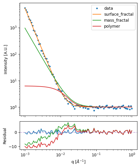
The residuals (differences between the model and data) provide a key way to assess the quality of the fits. A good fit should show residuals that:
Are randomly scattered around zero
Have no clear systematic trends or patterns
Are roughly within ±2-3 standard deviations of zero
Let’s plot the residuals for the first sample to assess the quality of our surface fractal fits:
Adding Model Selection to the Pipeline#
Okay, now to the hard part. We’ve fit the data, but we need to assess which model is best for each measurement. AutoSAS has a number of built in model selection tools for making this decision:
Bayesian Information Criterion (BIC) - Balances model complexity with goodness of fit
Akaike Information Criterion (AIC) - Similar to BIC but penalizes complexity less
Probability-based selection - Uses Bayesian probability theory to calculate model likelihoods
Chi-squared test - Compares the goodness of fit between models
We’ll use the Chi-square option for this demonstration
[47]:
from AFL.double_agent.AutoSAS import ModelSelectBestChiSq

with Pipeline() as autosas_pipeline2:
    AutoSAS(
        sas_variable='I',
        sas_err_variable='dI',
        q_variable = 'q',
        output_prefix='fit',
        model_inputs=model_inputs,
    )

    ModelSelectBestChiSq(
        all_chisq_var='fit_all_chisq',
        model_names_var='models',
        sample_dim='sample',
        output_prefix='BestChiSq',
    )
autosas_pipeline2.print()
PipelineOp                               input_variable ---> output_variable
----------                               -----------------------------------
0  ) <AutoSAS>                           ['q', 'I', 'dI'] ---> ['fit_all_chisq']
1  ) <ModelSelection_BestChiSq>          ['fit_all_chisq', 'models'] ---> ['BestChiSq_labels', 'BestChiSq_label_names']

Input Variables
---------------
0) q
1) I
2) dI
3) models

Output Variables
----------------
0) BestChiSq_labels
1) BestChiSq_label_names
[48]:
ds_result2 = autosas_pipeline2.calculate(ds_result)
ds_result2
[48]:
<xarray.Dataset> Size: 205kB
Dimensions:                    (sample: 30, q: 100, models: 3,
                                surface_fractal_params: 3,
                                mass_fractal_params: 3, polymer_params: 3,
                                fit_q_surface_fractal: 100,
                                fit_q_mass_fractal: 100, fit_q_polymer: 100)
Coordinates:
  * q                          (q) float64 800B 0.001 0.001072 ... 0.9326 1.0
  * models                     (models) <U15 180B 'surface_fractal' ... 'poly...
  * surface_fractal_params     (surface_fractal_params) <U26 312B 'surface_fr...
  * mass_fractal_params        (mass_fractal_params) <U23 276B 'mass_fractal_...
  * polymer_params             (polymer_params) <U18 216B 'polymer_scale' ......
  * fit_q_surface_fractal      (fit_q_surface_fractal) float64 800B 0.001 ......
  * fit_q_mass_fractal         (fit_q_mass_fractal) float64 800B 0.001 ... 1.0
  * fit_q_polymer              (fit_q_polymer) float64 800B 0.001 ... 1.0
Dimensions without coordinates: sample
Data variables: (12/21)
    I                          (sample, q) float64 24kB 5.465e+03 ... 1.002
    dI                         (sample, q) float64 24kB 545.9 429.3 ... 0.09923
    model                      (sample) object 240B 'surface_fractal' ... 'ma...
    sas_fit_sample             (sample) int64 240B 0 1 2 3 4 ... 25 26 27 28 29
    fit_all_chisq              (sample, models) float64 720B 1.023 ... 27.2
    probabilities              (sample, models) float64 720B 0.01182 ... 0.00...
    ...                         ...
    residuals_mass_fractal     (sample, fit_q_mass_fractal) float64 24kB -8.2...
    fit_I_polymer              (sample, fit_q_polymer) float64 24kB 6.219 ......
    residuals_polymer          (sample, fit_q_polymer) float64 24kB -10.0 ......
    BestChiSq_labels           (sample) int64 240B 0 1 0 1 2 0 0 ... 2 1 2 1 2 1
    BestChiSq_ChiSq            (sample) float64 240B 1.023 0.9502 ... 1.086
BestChiSq_label_names (sample) <U15 2kB 'surface_fractal' ... 'mass_...- sample: 30
- q: 100
- models: 3
- surface_fractal_params: 3
- mass_fractal_params: 3
- polymer_params: 3
- fit_q_surface_fractal: 100
- fit_q_mass_fractal: 100
- fit_q_polymer: 100
- q(q)float640.001 0.001072 ... 0.9326 1.0
array([0.001 , 0.001072, 0.00115 , 0.001233, 0.001322, 0.001417, 0.00152 , 0.00163 , 0.001748, 0.001874, 0.002009, 0.002154, 0.00231 , 0.002477, 0.002656, 0.002848, 0.003054, 0.003275, 0.003511, 0.003765, 0.004037, 0.004329, 0.004642, 0.004977, 0.005337, 0.005722, 0.006136, 0.006579, 0.007055, 0.007565, 0.008111, 0.008697, 0.009326, 0.01 , 0.010723, 0.011498, 0.012328, 0.013219, 0.014175, 0.015199, 0.016298, 0.017475, 0.018738, 0.020092, 0.021544, 0.023101, 0.024771, 0.026561, 0.02848 , 0.030539, 0.032745, 0.035112, 0.037649, 0.04037 , 0.043288, 0.046416, 0.04977 , 0.053367, 0.057224, 0.061359, 0.065793, 0.070548, 0.075646, 0.081113, 0.086975, 0.09326 , 0.1 , 0.107227, 0.114976, 0.123285, 0.132194, 0.141747, 0.151991, 0.162975, 0.174753, 0.187382, 0.200923, 0.215443, 0.231013, 0.247708, 0.265609, 0.284804, 0.305386, 0.327455, 0.351119, 0.376494, 0.403702, 0.432876, 0.464159, 0.497702, 0.53367 , 0.572237, 0.613591, 0.657933, 0.70548 , 0.756463, 0.811131, 0.869749, 0.932603, 1. ]) - models(models)<U15'surface_fractal' ... 'polymer'
array(['surface_fractal', 'mass_fractal', 'polymer'], dtype='<U15')
- surface_fractal_params(surface_fractal_params)<U26'surface_fractal_power' ... 'sur...
array(['surface_fractal_power', 'surface_fractal_scale', 'surface_fractal_background'], dtype='<U26') - mass_fractal_params(mass_fractal_params)<U23'mass_fractal_power' ... 'mass_f...
array(['mass_fractal_power', 'mass_fractal_scale', 'mass_fractal_background'], dtype='<U23') - polymer_params(polymer_params)<U18'polymer_scale' ... 'polymer_bac...
array(['polymer_scale', 'polymer_rg', 'polymer_background'], dtype='<U18')
- fit_q_surface_fractal(fit_q_surface_fractal)float640.001 0.001072 ... 0.9326 1.0
array([0.001 , 0.001072, 0.00115 , 0.001233, 0.001322, 0.001417, 0.00152 , 0.00163 , 0.001748, 0.001874, 0.002009, 0.002154, 0.00231 , 0.002477, 0.002656, 0.002848, 0.003054, 0.003275, 0.003511, 0.003765, 0.004037, 0.004329, 0.004642, 0.004977, 0.005337, 0.005722, 0.006136, 0.006579, 0.007055, 0.007565, 0.008111, 0.008697, 0.009326, 0.01 , 0.010723, 0.011498, 0.012328, 0.013219, 0.014175, 0.015199, 0.016298, 0.017475, 0.018738, 0.020092, 0.021544, 0.023101, 0.024771, 0.026561, 0.02848 , 0.030539, 0.032745, 0.035112, 0.037649, 0.04037 , 0.043288, 0.046416, 0.04977 , 0.053367, 0.057224, 0.061359, 0.065793, 0.070548, 0.075646, 0.081113, 0.086975, 0.09326 , 0.1 , 0.107227, 0.114976, 0.123285, 0.132194, 0.141747, 0.151991, 0.162975, 0.174753, 0.187382, 0.200923, 0.215443, 0.231013, 0.247708, 0.265609, 0.284804, 0.305386, 0.327455, 0.351119, 0.376494, 0.403702, 0.432876, 0.464159, 0.497702, 0.53367 , 0.572237, 0.613591, 0.657933, 0.70548 , 0.756463, 0.811131, 0.869749, 0.932603, 1. ]) - fit_q_mass_fractal(fit_q_mass_fractal)float640.001 0.001072 ... 0.9326 1.0
array([0.001 , 0.001072, 0.00115 , 0.001233, 0.001322, 0.001417, 0.00152 , 0.00163 , 0.001748, 0.001874, 0.002009, 0.002154, 0.00231 , 0.002477, 0.002656, 0.002848, 0.003054, 0.003275, 0.003511, 0.003765, 0.004037, 0.004329, 0.004642, 0.004977, 0.005337, 0.005722, 0.006136, 0.006579, 0.007055, 0.007565, 0.008111, 0.008697, 0.009326, 0.01 , 0.010723, 0.011498, 0.012328, 0.013219, 0.014175, 0.015199, 0.016298, 0.017475, 0.018738, 0.020092, 0.021544, 0.023101, 0.024771, 0.026561, 0.02848 , 0.030539, 0.032745, 0.035112, 0.037649, 0.04037 , 0.043288, 0.046416, 0.04977 , 0.053367, 0.057224, 0.061359, 0.065793, 0.070548, 0.075646, 0.081113, 0.086975, 0.09326 , 0.1 , 0.107227, 0.114976, 0.123285, 0.132194, 0.141747, 0.151991, 0.162975, 0.174753, 0.187382, 0.200923, 0.215443, 0.231013, 0.247708, 0.265609, 0.284804, 0.305386, 0.327455, 0.351119, 0.376494, 0.403702, 0.432876, 0.464159, 0.497702, 0.53367 , 0.572237, 0.613591, 0.657933, 0.70548 , 0.756463, 0.811131, 0.869749, 0.932603, 1. ]) - fit_q_polymer(fit_q_polymer)float640.001 0.001072 ... 0.9326 1.0
array([0.001   , 0.001072, 0.00115 , 0.001233, 0.001322, 0.001417, 0.00152 ,
       0.00163 , 0.001748, 0.001874, 0.002009, 0.002154, 0.00231 , 0.002477,
       0.002656, 0.002848, 0.003054, 0.003275, 0.003511, 0.003765, 0.004037,
       0.004329, 0.004642, 0.004977, 0.005337, 0.005722, 0.006136, 0.006579,
       0.007055, 0.007565, 0.008111, 0.008697, 0.009326, 0.01    , 0.010723,
       0.011498, 0.012328, 0.013219, 0.014175, 0.015199, 0.016298, 0.017475,
       0.018738, 0.020092, 0.021544, 0.023101, 0.024771, 0.026561, 0.02848 ,
       0.030539, 0.032745, 0.035112, 0.037649, 0.04037 , 0.043288, 0.046416,
       0.04977 , 0.053367, 0.057224, 0.061359, 0.065793, 0.070548, 0.075646,
       0.081113, 0.086975, 0.09326 , 0.1     , 0.107227, 0.114976, 0.123285,
       0.132194, 0.141747, 0.151991, 0.162975, 0.174753, 0.187382, 0.200923,
       0.215443, 0.231013, 0.247708, 0.265609, 0.284804, 0.305386, 0.327455,
       0.351119, 0.376494, 0.403702, 0.432876, 0.464159, 0.497702, 0.53367 ,
       0.572237, 0.613591, 0.657933, 0.70548 , 0.756463, 0.811131, 0.869749,
       0.932603, 1.      ])
- I(sample, q)float645.465e+03 4.598e+03 ... 1.1 1.002
array([[5.46461639e+03, 4.59795217e+03, 3.85947764e+03, ..., 8.23637450e-01, 1.08891674e+00, 8.86408253e-01], [1.14146226e+04, 1.20480054e+04, 9.60389049e+03, ..., 1.09249128e+00, 1.03151090e+00, 1.02766190e+00], [3.38673256e+03, 2.48217196e+03, 2.22022900e+03, ..., 1.16251134e+00, 1.01348467e+00, 1.15549165e+00], ..., [2.33984274e+04, 2.43947831e+04, 2.05533255e+04, ..., 1.04267181e+00, 9.85962747e-01, 9.07216458e-01], [2.09634325e+00, 2.08464279e+00, 1.81224765e+00, ..., 1.10735048e+00, 9.92568176e-01, 9.57666868e-01], [1.14052557e+04, 7.68845857e+03, 7.42318078e+03, ..., 1.03875573e+00, 1.10006506e+00, 1.00202285e+00]]) - dI(sample, q)float64545.9 429.3 ... 0.09923 0.09923
array([[5.45853473e+02, 4.29328308e+02, 3.42588723e+02, ..., 9.70709140e-02, 9.70708823e-02, 9.70708568e-02], [1.34833750e+03, 1.10406203e+03, 9.14697444e+02, ..., 1.00109160e-01, 1.00106587e-01, 1.00104428e-01], [3.10385847e+02, 2.45619675e+02, 1.97113531e+02, ..., 9.93385928e-02, 9.93385623e-02, 9.93385376e-02], ..., [2.78764336e+03, 2.26312770e+03, 1.86001084e+03, ..., 9.80268288e-02, 9.80242931e-02, 9.80221832e-02], [2.04875154e-01, 2.04855122e-01, 2.04833121e-01, ..., 1.02022577e-01, 1.02022027e-01, 1.02021575e-01], [1.15537649e+03, 9.47070166e+02, 7.85415799e+02, ..., 9.92344457e-02, 9.92320281e-02, 9.92299984e-02]]) - model(sample)object'surface_fractal' ... 'mass_frac...
array(['surface_fractal', 'mass_fractal', 'surface_fractal', 'mass_fractal', 'polymer_excl_volume', 'surface_fractal', 'surface_fractal', 'surface_fractal', 'polymer_excl_volume', 'mass_fractal', 'mass_fractal', 'polymer_excl_volume', 'polymer_excl_volume', 'mass_fractal', 'surface_fractal', 'surface_fractal', 'mass_fractal', 'surface_fractal', 'surface_fractal', 'surface_fractal', 'polymer_excl_volume', 'polymer_excl_volume', 'polymer_excl_volume', 'mass_fractal', 'polymer_excl_volume', 'mass_fractal', 'polymer_excl_volume', 'mass_fractal', 'polymer_excl_volume', 'mass_fractal'], dtype=object) - sas_fit_sample(sample)int640 1 2 3 4 5 6 ... 24 25 26 27 28 29
- name :
- AutoSAS
- input_variable :
- ['q', 'I', 'dI']
- output_variable :
- ['fit_all_chisq']
- input_prefix :
- None
- output_prefix :
- fit
- server_id :
- None
- fit_method :
- None
- model_inputs :
- [{'name': 'surface_fractal', 'sasmodel': 'power_law', 'q_min': 0.001, 'q_max': 1.0, 'fit_params': {'power': {'value': 4, 'bounds': (3, 4)}, 'scale': {'value': 1.0, 'bounds': (1e-06, 0.001)}, 'background': {'value': 1.0}}}, {'name': 'mass_fractal', 'sasmodel': 'power_law', 'q_min': 0.001, 'q_max': 1.0, 'fit_params': {'power': {'value': 4, 'bounds': (1.7, 3)}, 'scale': {'value': 1.0, 'bounds': (0.0001, 0.1)}, 'background': {'value': 1.0}}}, {'name': 'polymer', 'sasmodel': 'polymer_excl_volume', 'q_min': 0.001, 'q_max': 1.0, 'fit_params': {'scale': {'value': 1.0, 'bounds': (0.01, 100.0)}, 'rg': {'value': 60.0, 'bounds': (10, 150)}, 'background': {'value': 1.0}}}]
- results :
- {}
- q_variable :
- q
- sas_variable :
- I
- sas_err_variable :
- dI
- resolution :
- None
- sample_dim :
- sample
- model_dim :
- models
- q_min :
- None
- q_max :
- None
array([ 0, 1, 2, 3, 4, 5, 6, 7, 8, 9, 10, 11, 12, 13, 14, 15, 16, 17, 18, 19, 20, 21, 22, 23, 24, 25, 26, 27, 28, 29]) - fit_all_chisq(sample, models)float641.023 14.07 27.32 ... 1.086 27.2
- fit_calc_id :
- ASAS-44f48a96-589b-473b-8411-8df15b6c95a4
- name :
- AutoSAS
- input_variable :
- ['q', 'I', 'dI']
- output_variable :
- ['fit_all_chisq']
- input_prefix :
- None
- output_prefix :
- fit
- server_id :
- None
- fit_method :
- None
- model_inputs :
- [{'name': 'surface_fractal', 'sasmodel': 'power_law', 'q_min': 0.001, 'q_max': 1.0, 'fit_params': {'power': {'value': 4, 'bounds': (3, 4)}, 'scale': {'value': 1.0, 'bounds': (1e-06, 0.001)}, 'background': {'value': 1.0}}}, {'name': 'mass_fractal', 'sasmodel': 'power_law', 'q_min': 0.001, 'q_max': 1.0, 'fit_params': {'power': {'value': 4, 'bounds': (1.7, 3)}, 'scale': {'value': 1.0, 'bounds': (0.0001, 0.1)}, 'background': {'value': 1.0}}}, {'name': 'polymer', 'sasmodel': 'polymer_excl_volume', 'q_min': 0.001, 'q_max': 1.0, 'fit_params': {'scale': {'value': 1.0, 'bounds': (0.01, 100.0)}, 'rg': {'value': 60.0, 'bounds': (10, 150)}, 'background': {'value': 1.0}}}]
- results :
- {}
- q_variable :
- q
- sas_variable :
- I
- sas_err_variable :
- dI
- resolution :
- None
- sample_dim :
- sample
- model_dim :
- models
- q_min :
- None
- q_max :
- None
array([[1.02275423e+00, 1.40722782e+01, 2.73224420e+01], [4.09722407e+00, 9.50171680e-01, 2.63673388e+01], [1.05413472e+00, 1.36841369e+01, 2.72866689e+01], [1.14629265e+00, 1.04990624e+00, 3.17019675e+01], [6.96376204e+05, 1.35878440e+02, 1.18324132e+00], [1.08126923e+00, 1.19570931e+01, 2.58392185e+01], [8.36611432e-01, 1.21540498e+01, 2.69767485e+01], [8.92581487e-01, 1.12844843e+01, 2.53700558e+01], [7.43408306e+05, 1.44644370e+02, 1.11691133e+00], [4.08984295e+00, 9.12932757e-01, 2.64968640e+01], [1.32050220e+00, 9.75581038e-01, 3.07720967e+01], [7.06812364e+05, 1.37343734e+02, 9.18066715e-01], [7.71372671e+05, 1.56599393e+02, 9.73842068e-01], [1.57930523e+00, 1.01924014e+00, 3.04306793e+01], [9.31217832e-01, 1.24766894e+01, 2.55126991e+01], [9.27394330e-01, 1.03076313e+01, 2.44011743e+01], [4.01568675e+00, 8.51332910e-01, 2.83843343e+01], [1.07638344e+00, 1.05327569e+01, 2.38169213e+01], [8.71404947e-01, 8.93694309e+00, 2.19797127e+01], [1.08324978e+00, 9.81511077e+00, 2.41165279e+01], [7.36691528e+05, 1.47836036e+02, 1.09358942e+00], [7.15150775e+05, 1.38734930e+02, 1.10718714e+00], [7.28863488e+05, 1.47481645e+02, 9.61265988e-01], [2.05590837e+00, 1.13113537e+00, 2.80256684e+01], [7.30479177e+05, 1.44870136e+02, 1.03919799e+00], [1.23729309e+00, 8.66385752e-01, 2.81719466e+01], [7.49889915e+05, 1.51181543e+02, 9.99128955e-01], [2.42291207e+00, 1.16555890e+00, 3.01412948e+01], [7.08550329e+05, 1.41412767e+02, 1.08373657e+00], [4.75962943e+00, 1.08625395e+00, 2.72039930e+01]]) - probabilities(sample, models)float640.01182 0.9238 ... 0.9984 0.001121
- name :
- AutoSAS
- input_variable :
- ['q', 'I', 'dI']
- output_variable :
- ['fit_all_chisq']
- input_prefix :
- None
- output_prefix :
- fit
- server_id :
- None
- fit_method :
- None
- model_inputs :
- [{'name': 'surface_fractal', 'sasmodel': 'power_law', 'q_min': 0.001, 'q_max': 1.0, 'fit_params': {'power': {'value': 4, 'bounds': (3, 4)}, 'scale': {'value': 1.0, 'bounds': (1e-06, 0.001)}, 'background': {'value': 1.0}}}, {'name': 'mass_fractal', 'sasmodel': 'power_law', 'q_min': 0.001, 'q_max': 1.0, 'fit_params': {'power': {'value': 4, 'bounds': (1.7, 3)}, 'scale': {'value': 1.0, 'bounds': (0.0001, 0.1)}, 'background': {'value': 1.0}}}, {'name': 'polymer', 'sasmodel': 'polymer_excl_volume', 'q_min': 0.001, 'q_max': 1.0, 'fit_params': {'scale': {'value': 1.0, 'bounds': (0.01, 100.0)}, 'rg': {'value': 60.0, 'bounds': (10, 150)}, 'background': {'value': 1.0}}}]
- results :
- {}
- q_variable :
- q
- sas_variable :
- I
- sas_err_variable :
- dI
- resolution :
- None
- sample_dim :
- sample
- model_dim :
- models
- q_min :
- None
- q_max :
- None
array([[1.18241649e-02, 9.23820654e-01, 6.43551809e-02], [1.23607135e-03, 9.96341125e-01, 2.42280337e-03], [8.23266617e-03, 9.40641961e-01, 5.11253726e-02], [4.27533439e-01, 5.72377505e-01, 8.90553923e-05], [0.00000000e+00, 1.73073808e-64, 1.00000000e+00], [1.49740488e-03, 9.57828584e-01, 4.06740111e-02], [3.55950627e-03, 9.80632154e-01, 1.58083397e-02], [9.17293426e-04, 9.47240896e-01, 5.18418105e-02], [0.00000000e+00, 1.78346827e-68, 1.00000000e+00], [1.27297309e-02, 9.85285111e-01, 1.98515819e-03], [3.07295385e-01, 6.92659281e-01, 4.53336987e-05], [0.00000000e+00, 2.87852843e-65, 1.00000000e+00], [0.00000000e+00, 9.22602333e-74, 1.00000000e+00], [2.61966631e-01, 7.37981212e-01, 5.21571954e-05], [3.16094856e-03, 9.03018069e-01, 9.38209827e-02], [3.49580420e-04, 9.71200269e-01, 2.84501501e-02], [1.29078990e-02, 9.86763088e-01, 3.29012466e-04], [3.03155123e-04, 7.98369591e-01, 2.01327254e-01], [8.19662930e-05, 9.22293393e-01, 7.76246408e-02], [1.01633723e-04, 5.47733346e-01, 4.52165021e-01], [0.00000000e+00, 7.95457604e-70, 1.00000000e+00], [0.00000000e+00, 6.45880860e-66, 1.00000000e+00], [0.00000000e+00, 8.57179161e-70, 1.00000000e+00], [1.74573275e-01, 8.24542384e-01, 8.84340955e-04], [0.00000000e+00, 1.81958266e-68, 1.00000000e+00], [3.19004059e-01, 6.80291474e-01, 7.04467341e-04], [0.00000000e+00, 2.68265729e-71, 1.00000000e+00], [1.02787938e-01, 8.97121386e-01, 9.06757543e-05], [0.00000000e+00, 5.10032208e-67, 1.00000000e+00], [5.20020767e-04, 9.98358893e-01, 1.12108653e-03]]) - surface_fractal_fit_val(surface_fractal_params, sample)float643.243 3.0 3.163 3.0 ... 1.0 1.0 1.0
- fit_calc_id :
- ASAS-44f48a96-589b-473b-8411-8df15b6c95a4
- name :
- AutoSAS
- input_variable :
- ['q', 'I', 'dI']
- output_variable :
- ['fit_all_chisq']
- input_prefix :
- None
- output_prefix :
- fit
- server_id :
- None
- fit_method :
- None
- model_inputs :
- [{'name': 'surface_fractal', 'sasmodel': 'power_law', 'q_min': 0.001, 'q_max': 1.0, 'fit_params': {'power': {'value': 4, 'bounds': (3, 4)}, 'scale': {'value': 1.0, 'bounds': (1e-06, 0.001)}, 'background': {'value': 1.0}}}, {'name': 'mass_fractal', 'sasmodel': 'power_law', 'q_min': 0.001, 'q_max': 1.0, 'fit_params': {'power': {'value': 4, 'bounds': (1.7, 3)}, 'scale': {'value': 1.0, 'bounds': (0.0001, 0.1)}, 'background': {'value': 1.0}}}, {'name': 'polymer', 'sasmodel': 'polymer_excl_volume', 'q_min': 0.001, 'q_max': 1.0, 'fit_params': {'scale': {'value': 1.0, 'bounds': (0.01, 100.0)}, 'rg': {'value': 60.0, 'bounds': (10, 150)}, 'background': {'value': 1.0}}}]
- results :
- {}
- q_variable :
- q
- sas_variable :
- I
- sas_err_variable :
- dI
- resolution :
- None
- sample_dim :
- sample
- model_dim :
- models
- q_min :
- None
- q_max :
- None
array([[3.24265739e+00, 3.00000000e+00, 3.16252070e+00, 3.00000000e+00, 3.00000000e+00, 3.08615609e+00, 3.15552503e+00, 3.05113167e+00, 3.00000000e+00, 3.00000000e+00, 3.00000000e+00, 3.00000000e+00, 3.00000000e+00, 3.00000000e+00, 3.25242366e+00, 3.03037286e+00, 3.00000000e+00, 3.00000000e+00, 3.00000000e+00, 3.00000000e+00, 3.00000000e+00, 3.00000000e+00, 3.00000000e+00, 3.00000000e+00, 3.00000000e+00, 3.00000000e+00, 3.00000000e+00, 3.00000000e+00, 3.00000000e+00, 3.00000000e+00], [1.00000000e-06, 1.88805902e-05, 1.00000000e-06, 8.07491165e-05, 1.00000000e-06, 1.00000000e-06, 1.24393004e-06, 1.00000000e-06, 1.00000000e-06, 2.18202275e-05, 6.10328588e-05, 1.00000000e-06, 1.00000000e-06, 5.96185299e-05, 1.11492212e-06, 1.00000000e-06, 2.25881511e-05, 1.00000000e-06, 1.00000000e-06, 1.00000000e-06, 1.00000000e-06, 1.00000000e-06, 1.00000000e-06, 5.01149203e-05, 1.00000000e-06, 6.92824955e-05, 1.00000000e-06, 3.59572491e-05, 1.00000000e-06, 1.64517485e-05], [1.00000000e+00, 1.00000000e+00, 1.00000000e+00, 1.00000000e+00, 1.00000000e+00, 1.00000000e+00, 1.00000000e+00, 1.00000000e+00, 1.00000000e+00, 1.00000000e+00, 1.00000000e+00, 1.00000000e+00, 1.00000000e+00, 1.00000000e+00, 1.00000000e+00, 1.00000000e+00, 1.00000000e+00, 1.00000000e+00, 1.00000000e+00, 1.00000000e+00, 1.00000000e+00, 1.00000000e+00, 1.00000000e+00, 1.00000000e+00, 1.00000000e+00, 1.00000000e+00, 1.00000000e+00, 1.00000000e+00, 1.00000000e+00, 1.00000000e+00]]) - surface_fractal_fit_err(surface_fractal_params, sample)float640.0227 0.01792 0.02407 ... 0.0 0.0
- fit_calc_id :
- ASAS-44f48a96-589b-473b-8411-8df15b6c95a4
- name :
- AutoSAS
- input_variable :
- ['q', 'I', 'dI']
- output_variable :
- ['fit_all_chisq']
- input_prefix :
- None
- output_prefix :
- fit
- server_id :
- None
- fit_method :
- None
- model_inputs :
- [{'name': 'surface_fractal', 'sasmodel': 'power_law', 'q_min': 0.001, 'q_max': 1.0, 'fit_params': {'power': {'value': 4, 'bounds': (3, 4)}, 'scale': {'value': 1.0, 'bounds': (1e-06, 0.001)}, 'background': {'value': 1.0}}}, {'name': 'mass_fractal', 'sasmodel': 'power_law', 'q_min': 0.001, 'q_max': 1.0, 'fit_params': {'power': {'value': 4, 'bounds': (1.7, 3)}, 'scale': {'value': 1.0, 'bounds': (0.0001, 0.1)}, 'background': {'value': 1.0}}}, {'name': 'polymer', 'sasmodel': 'polymer_excl_volume', 'q_min': 0.001, 'q_max': 1.0, 'fit_params': {'scale': {'value': 1.0, 'bounds': (0.01, 100.0)}, 'rg': {'value': 60.0, 'bounds': (10, 150)}, 'background': {'value': 1.0}}}]
- results :
- {}
- q_variable :
- q
- sas_variable :
- I
- sas_err_variable :
- dI
- resolution :
- None
- sample_dim :
- sample
- model_dim :
- models
- q_min :
- None
- q_max :
- None
array([[2.27048704e-02, 1.79223126e-02, 2.40659471e-02, 1.30755205e-02, 7.27887423e-04, 2.55743991e-02, 2.29994739e-02, 2.63328387e-02, 7.04419584e-04, 1.73100251e-02, 1.37324240e-02, 7.22326241e-04, 6.91839641e-04, 1.39774626e-02, 2.28313482e-02, 2.70634988e-02, 1.68284235e-02, 2.78456852e-02, 2.78247365e-02, 2.77249316e-02, 7.07711080e-04, 7.18157333e-04, 7.11603537e-04, 1.46252174e-02, 7.10825868e-04, 1.38115165e-02, 7.01610295e-04, 1.51664322e-02, 7.21627230e-04, 1.82691043e-02], [1.30712675e-07, 1.99407460e-06, 1.39863344e-07, 5.68296258e-06, 4.93677731e-09, 1.49719861e-07, 1.64556199e-07, 1.55220020e-07, 4.77760508e-09, 2.21210410e-06, 4.59230273e-06, 4.89904463e-09, 4.69228908e-09, 4.58996792e-06, 1.45467891e-07, 1.59749280e-07, 2.22355435e-06, 1.64812550e-07, 1.64903795e-07, 1.64396226e-07, 4.79992379e-09, 4.87077236e-09, 4.82632551e-09, 4.07911051e-06, 4.82106811e-09, 5.20163539e-06, 4.75856119e-09, 3.10007783e-06, 4.89431125e-09, 1.77906351e-06], [0.00000000e+00, 0.00000000e+00, 0.00000000e+00, 0.00000000e+00, 0.00000000e+00, 0.00000000e+00, 0.00000000e+00, 0.00000000e+00, 0.00000000e+00, 0.00000000e+00, 0.00000000e+00, 0.00000000e+00, 0.00000000e+00, 0.00000000e+00, 0.00000000e+00, 0.00000000e+00, 0.00000000e+00, 0.00000000e+00, 0.00000000e+00, 0.00000000e+00, 0.00000000e+00, 0.00000000e+00, 0.00000000e+00, 0.00000000e+00, 0.00000000e+00, 0.00000000e+00, 0.00000000e+00, 0.00000000e+00, 0.00000000e+00, 0.00000000e+00]]) - mass_fractal_fit_val(mass_fractal_params, sample)float642.327 2.708 2.263 ... 1.0 1.0 1.0
- fit_calc_id :
- ASAS-44f48a96-589b-473b-8411-8df15b6c95a4
- name :
- AutoSAS
- input_variable :
- ['q', 'I', 'dI']
- output_variable :
- ['fit_all_chisq']
- input_prefix :
- None
- output_prefix :
- fit
- server_id :
- None
- fit_method :
- None
- model_inputs :
- [{'name': 'surface_fractal', 'sasmodel': 'power_law', 'q_min': 0.001, 'q_max': 1.0, 'fit_params': {'power': {'value': 4, 'bounds': (3, 4)}, 'scale': {'value': 1.0, 'bounds': (1e-06, 0.001)}, 'background': {'value': 1.0}}}, {'name': 'mass_fractal', 'sasmodel': 'power_law', 'q_min': 0.001, 'q_max': 1.0, 'fit_params': {'power': {'value': 4, 'bounds': (1.7, 3)}, 'scale': {'value': 1.0, 'bounds': (0.0001, 0.1)}, 'background': {'value': 1.0}}}, {'name': 'polymer', 'sasmodel': 'polymer_excl_volume', 'q_min': 0.001, 'q_max': 1.0, 'fit_params': {'scale': {'value': 1.0, 'bounds': (0.01, 100.0)}, 'rg': {'value': 60.0, 'bounds': (10, 150)}, 'background': {'value': 1.0}}}]
- results :
- {}
- q_variable :
- q
- sas_variable :
- I
- sas_err_variable :
- dI
- resolution :
- None
- sample_dim :
- sample
- model_dim :
- models
- q_min :
- None
- q_max :
- None
array([[2.32667232e+00, 2.70771805e+00, 2.26272645e+00, 2.95928814e+00, 1.70000000e+00, 2.20397864e+00, 2.29631053e+00, 2.17898167e+00, 1.70000000e+00, 2.72327751e+00, 2.90766327e+00, 1.70000000e+00, 1.70000000e+00, 2.89774061e+00, 2.35502215e+00, 2.16469122e+00, 2.72861467e+00, 2.13300103e+00, 2.13477745e+00, 2.14056161e+00, 1.70000000e+00, 1.70000000e+00, 1.70000000e+00, 2.86340973e+00, 1.70000000e+00, 2.91737002e+00, 1.70000000e+00, 2.81452282e+00, 1.70000000e+00, 2.68510041e+00], [1.00000000e-04, 1.00000000e-04, 1.00000000e-04, 1.00000000e-04, 1.00000000e-04, 1.00000000e-04, 1.00000000e-04, 1.00000000e-04, 1.00000000e-04, 1.04785464e-04, 1.00000000e-04, 1.00000000e-04, 1.00000000e-04, 1.03066892e-04, 1.00000000e-04, 1.00000000e-04, 1.05075202e-04, 1.00000000e-04, 1.00000000e-04, 1.00000000e-04, 1.00000000e-04, 1.00000000e-04, 1.00000000e-04, 1.04777291e-04, 1.00000000e-04, 1.07215235e-04, 1.00000000e-04, 1.00000000e-04, 1.00000000e-04, 1.00000000e-04], [1.00000000e+00, 1.00000000e+00, 1.00000000e+00, 1.00000000e+00, 1.00000000e+00, 1.00000000e+00, 1.00000000e+00, 1.00000000e+00, 1.00000000e+00, 1.00000000e+00, 1.00000000e+00, 1.00000000e+00, 1.00000000e+00, 1.00000000e+00, 1.00000000e+00, 1.00000000e+00, 1.00000000e+00, 1.00000000e+00, 1.00000000e+00, 1.00000000e+00, 1.00000000e+00, 1.00000000e+00, 1.00000000e+00, 1.00000000e+00, 1.00000000e+00, 1.00000000e+00, 1.00000000e+00, 1.00000000e+00, 1.00000000e+00, 1.00000000e+00]]) - mass_fractal_fit_err(mass_fractal_params, sample)float640.03115 0.01507 0.03165 ... 0.0 0.0
- fit_calc_id :
- ASAS-44f48a96-589b-473b-8411-8df15b6c95a4
- name :
- AutoSAS
- input_variable :
- ['q', 'I', 'dI']
- output_variable :
- ['fit_all_chisq']
- input_prefix :
- None
- output_prefix :
- fit
- server_id :
- None
- fit_method :
- None
- model_inputs :
- [{'name': 'surface_fractal', 'sasmodel': 'power_law', 'q_min': 0.001, 'q_max': 1.0, 'fit_params': {'power': {'value': 4, 'bounds': (3, 4)}, 'scale': {'value': 1.0, 'bounds': (1e-06, 0.001)}, 'background': {'value': 1.0}}}, {'name': 'mass_fractal', 'sasmodel': 'power_law', 'q_min': 0.001, 'q_max': 1.0, 'fit_params': {'power': {'value': 4, 'bounds': (1.7, 3)}, 'scale': {'value': 1.0, 'bounds': (0.0001, 0.1)}, 'background': {'value': 1.0}}}, {'name': 'polymer', 'sasmodel': 'polymer_excl_volume', 'q_min': 0.001, 'q_max': 1.0, 'fit_params': {'scale': {'value': 1.0, 'bounds': (0.01, 100.0)}, 'rg': {'value': 60.0, 'bounds': (10, 150)}, 'background': {'value': 1.0}}}]
- results :
- {}
- q_variable :
- q
- sas_variable :
- I
- sas_err_variable :
- dI
- resolution :
- None
- sample_dim :
- sample
- model_dim :
- models
- q_min :
- None
- q_max :
- None
array([[3.11538645e-02, 1.50731929e-02, 3.16536073e-02, 1.29313013e-02, 2.54503819e-02, 3.16613936e-02, 2.96995833e-02, 3.15895469e-02, 2.46166729e-02, 1.47327752e-02, 1.33044826e-02, 2.52264042e-02, 2.41889926e-02, 1.34897817e-02, 3.12569447e-02, 3.15930608e-02, 1.44385458e-02, 3.31186418e-02, 3.30138173e-02, 3.19064838e-02, 2.47254105e-02, 2.50868816e-02, 2.48625273e-02, 1.39016032e-02, 2.48696932e-02, 1.34768498e-02, 2.45398366e-02, 1.39221047e-02, 2.52168618e-02, 1.51065202e-02], [1.48852173e-05, 8.14818887e-06, 1.54933083e-05, 6.84638978e-06, 1.69408717e-05, 1.58106544e-05, 1.44407776e-05, 1.59900730e-05, 1.63857670e-05, 8.30277128e-06, 7.03419636e-06, 1.67913949e-05, 1.61012315e-05, 7.36494592e-06, 1.48565822e-05, 1.60709381e-05, 8.16838404e-06, 1.69550162e-05, 1.69592147e-05, 1.64106194e-05, 1.64580270e-05, 1.66985964e-05, 1.65493330e-05, 7.70810369e-06, 1.65545487e-05, 7.59938920e-06, 1.63348826e-05, 7.42614119e-06, 1.67852396e-05, 8.16621099e-06], [0.00000000e+00, 0.00000000e+00, 0.00000000e+00, 0.00000000e+00, 0.00000000e+00, 0.00000000e+00, 0.00000000e+00, 0.00000000e+00, 0.00000000e+00, 0.00000000e+00, 0.00000000e+00, 0.00000000e+00, 0.00000000e+00, 0.00000000e+00, 0.00000000e+00, 0.00000000e+00, 0.00000000e+00, 0.00000000e+00, 0.00000000e+00, 0.00000000e+00, 0.00000000e+00, 0.00000000e+00, 0.00000000e+00, 0.00000000e+00, 0.00000000e+00, 0.00000000e+00, 0.00000000e+00, 0.00000000e+00, 0.00000000e+00, 0.00000000e+00]]) - polymer_fit_val(polymer_params, sample)float645.258 40.23 4.006 ... 1.0 1.0 1.0
- fit_calc_id :
- ASAS-44f48a96-589b-473b-8411-8df15b6c95a4
- name :
- AutoSAS
- input_variable :
- ['q', 'I', 'dI']
- output_variable :
- ['fit_all_chisq']
- input_prefix :
- None
- output_prefix :
- fit
- server_id :
- None
- fit_method :
- None
- model_inputs :
- [{'name': 'surface_fractal', 'sasmodel': 'power_law', 'q_min': 0.001, 'q_max': 1.0, 'fit_params': {'power': {'value': 4, 'bounds': (3, 4)}, 'scale': {'value': 1.0, 'bounds': (1e-06, 0.001)}, 'background': {'value': 1.0}}}, {'name': 'mass_fractal', 'sasmodel': 'power_law', 'q_min': 0.001, 'q_max': 1.0, 'fit_params': {'power': {'value': 4, 'bounds': (1.7, 3)}, 'scale': {'value': 1.0, 'bounds': (0.0001, 0.1)}, 'background': {'value': 1.0}}}, {'name': 'polymer', 'sasmodel': 'polymer_excl_volume', 'q_min': 0.001, 'q_max': 1.0, 'fit_params': {'scale': {'value': 1.0, 'bounds': (0.01, 100.0)}, 'rg': {'value': 60.0, 'bounds': (10, 150)}, 'background': {'value': 1.0}}}]
- results :
- {}
- q_variable :
- q
- sas_variable :
- I
- sas_err_variable :
- dI
- resolution :
- None
- sample_dim :
- sample
- model_dim :
- models
- q_min :
- None
- q_max :
- None
array([[ 5.25833492, 40.22505817, 4.00558774, 100. , 1.04442146, 3.29761 , 4.8720121 , 3.06146257, 1.00713336, 44.27147743, 78.17551856, 1.02892542, 0.93875659, 100. , 6.08637701, 2.94546786, 45.0702793 , 2.50345304, 2.73405192, 2.70524025, 0.96785773, 1.03149347, 1.02593748, 71.97009094, 1.01287684, 100. , 0.94249659, 56.17376216, 1.04479582, 36.40920265], [150. , 150. , 150. , 150. , 51.06176077, 150. , 150. , 150. , 66.89120632, 150. , 150. , 56.50715476, 60.19825947, 150. , 150. , 150. , 150. , 150. , 150. , 150. , 57.51120818, 65.91860794, 66.08437723, 150. , 51.03465948, 150. , 54.99540066, 150. , 57.39639901, 150. ], [ 1. , 1. , 1. , 1. , 1. , 1. , 1. , 1. , 1. , 1. , 1. , 1. , 1. , 1. , 1. , 1. , 1. , 1. , 1. , 1. , 1. , 1. , 1. , 1. , 1. , 1. , 1. , 1. , 1. , 1. ]]) - polymer_fit_err(polymer_params, sample)float640.557 3.071 0.4278 ... 0.0 0.0 0.0
- fit_calc_id :
- ASAS-44f48a96-589b-473b-8411-8df15b6c95a4
- name :
- AutoSAS
- input_variable :
- ['q', 'I', 'dI']
- output_variable :
- ['fit_all_chisq']
- input_prefix :
- None
- output_prefix :
- fit
- server_id :
- None
- fit_method :
- None
- model_inputs :
- [{'name': 'surface_fractal', 'sasmodel': 'power_law', 'q_min': 0.001, 'q_max': 1.0, 'fit_params': {'power': {'value': 4, 'bounds': (3, 4)}, 'scale': {'value': 1.0, 'bounds': (1e-06, 0.001)}, 'background': {'value': 1.0}}}, {'name': 'mass_fractal', 'sasmodel': 'power_law', 'q_min': 0.001, 'q_max': 1.0, 'fit_params': {'power': {'value': 4, 'bounds': (1.7, 3)}, 'scale': {'value': 1.0, 'bounds': (0.0001, 0.1)}, 'background': {'value': 1.0}}}, {'name': 'polymer', 'sasmodel': 'polymer_excl_volume', 'q_min': 0.001, 'q_max': 1.0, 'fit_params': {'scale': {'value': 1.0, 'bounds': (0.01, 100.0)}, 'rg': {'value': 60.0, 'bounds': (10, 150)}, 'background': {'value': 1.0}}}]
- results :
- {}
- q_variable :
- q
- sas_variable :
- I
- sas_err_variable :
- dI
- resolution :
- None
- sample_dim :
- sample
- model_dim :
- models
- q_min :
- None
- q_max :
- None
array([[ 0.55701407, 3.07117713, 0.42778412, 8.69419771, 0.03408775, 0.33168065, 0.46750051, 0.30125613, 0.03525603, 3.39906167, 6.95871167, 0.03454602, 0.03374983, 6.96250167, 0.63187833, 0.28329694, 3.39953852, 0.25694993, 0.25926761, 0.25897734, 0.03405919, 0.03578345, 0.03549022, 6.14599674, 0.03336914, 7.93845586, 0.03350642, 4.68010318, 0.03472009, 2.74813752], [ 8.43420851, 5.0489181 , 9.08329964, 5.2036293 , 3.21497204, 9.0828923 , 7.97555919, 9.20181048, 4.55893797, 5.00749523, 5.41144915, 3.59425279, 4.22852841, 4.24658521, 8.14522953, 9.14026989, 4.9375889 , 10.01209928, 9.33676861, 9.42076471, 3.90038145, 4.44092837, 4.44246663, 5.27284562, 3.29848751, 4.78430279, 3.83062797, 5.25408604, 3.66863617, 5.04400228], [ 0. , 0. , 0. , 0. , 0. , 0. , 0. , 0. , 0. , 0. , 0. , 0. , 0. , 0. , 0. , 0. , 0. , 0. , 0. , 0. , 0. , 0. , 0. , 0. , 0. , 0. , 0. , 0. , 0. , 0. ]]) - fit_I_surface_fractal(sample, fit_q_surface_fractal)float645.346e+03 4.264e+03 ... 1.0 1.0
- name :
- AutoSAS
- input_variable :
- ['q', 'I', 'dI']
- output_variable :
- ['fit_all_chisq']
- input_prefix :
- None
- output_prefix :
- fit
- server_id :
- None
- fit_method :
- None
- model_inputs :
- [{'name': 'surface_fractal', 'sasmodel': 'power_law', 'q_min': 0.001, 'q_max': 1.0, 'fit_params': {'power': {'value': 4, 'bounds': (3, 4)}, 'scale': {'value': 1.0, 'bounds': (1e-06, 0.001)}, 'background': {'value': 1.0}}}, {'name': 'mass_fractal', 'sasmodel': 'power_law', 'q_min': 0.001, 'q_max': 1.0, 'fit_params': {'power': {'value': 4, 'bounds': (1.7, 3)}, 'scale': {'value': 1.0, 'bounds': (0.0001, 0.1)}, 'background': {'value': 1.0}}}, {'name': 'polymer', 'sasmodel': 'polymer_excl_volume', 'q_min': 0.001, 'q_max': 1.0, 'fit_params': {'scale': {'value': 1.0, 'bounds': (0.01, 100.0)}, 'rg': {'value': 60.0, 'bounds': (10, 150)}, 'background': {'value': 1.0}}}]
- results :
- {}
- q_variable :
- q
- sas_variable :
- I
- sas_err_variable :
- dI
- resolution :
- None
- sample_dim :
- sample
- model_dim :
- models
- q_min :
- None
- q_max :
- None
array([[5.34630102e+03, 4.26394591e+03, 3.40075387e+03, ..., 1.00000157e+00, 1.00000125e+00, 1.00000100e+00], [1.88815902e+04, 1.53156289e+04, 1.24231676e+04, ..., 1.00002870e+00, 1.00002328e+00, 1.00001888e+00], [3.07399683e+03, 2.46549619e+03, 1.97748804e+03, ..., 1.00000155e+00, 1.00000125e+00, 1.00000100e+00], ..., [3.59582491e+04, 2.91670333e+04, 2.36584688e+04, ..., 1.00005465e+00, 1.00004433e+00, 1.00003596e+00], [1.00100000e+03, 8.12130831e+02, 6.58933225e+02, ..., 1.00000152e+00, 1.00000123e+00, 1.00000100e+00], [1.64527485e+04, 1.33455205e+04, 1.08251520e+04, ..., 1.00002501e+00, 1.00002028e+00, 1.00001645e+00]]) - residuals_surface_fractal(sample, fit_q_surface_fractal)float64-0.2168 -0.778 ... -1.008 -0.02022
- name :
- AutoSAS
- input_variable :
- ['q', 'I', 'dI']
- output_variable :
- ['fit_all_chisq']
- input_prefix :
- None
- output_prefix :
- fit
- server_id :
- None
- fit_method :
- None
- model_inputs :
- [{'name': 'surface_fractal', 'sasmodel': 'power_law', 'q_min': 0.001, 'q_max': 1.0, 'fit_params': {'power': {'value': 4, 'bounds': (3, 4)}, 'scale': {'value': 1.0, 'bounds': (1e-06, 0.001)}, 'background': {'value': 1.0}}}, {'name': 'mass_fractal', 'sasmodel': 'power_law', 'q_min': 0.001, 'q_max': 1.0, 'fit_params': {'power': {'value': 4, 'bounds': (1.7, 3)}, 'scale': {'value': 1.0, 'bounds': (0.0001, 0.1)}, 'background': {'value': 1.0}}}, {'name': 'polymer', 'sasmodel': 'polymer_excl_volume', 'q_min': 0.001, 'q_max': 1.0, 'fit_params': {'scale': {'value': 1.0, 'bounds': (0.01, 100.0)}, 'rg': {'value': 60.0, 'bounds': (10, 150)}, 'background': {'value': 1.0}}}]
- results :
- {}
- q_variable :
- q
- sas_variable :
- I
- sas_err_variable :
- dI
- resolution :
- None
- sample_dim :
- sample
- model_dim :
- models
- q_min :
- None
- q_max :
- None
array([[-2.16752990e-01, -7.77973996e-01, -1.33899259e+00, ..., 1.81685857e+00, -9.15985177e-01, 1.17020443e+00], [ 5.53790700e+00, 2.95963752e+00, 3.08219636e+00, ..., -9.23617634e-01, -3.14540965e-01, -2.76141815e-01], [-1.00757084e+00, -6.78926389e-02, -1.23147789e+00, ..., -1.63591791e+00, -1.35732062e-01, -1.56526014e+00], ..., [ 4.50553393e+00, 2.10869684e+00, 1.66942220e+00, ..., -4.34749911e-01, 1.43654008e-01, 9.46923398e-01], [ 4.87567006e+03, 3.95423936e+03, 3.20807969e+03, ..., -1.05220784e+00, 7.28573742e-02, 4.14952742e-01], [ 4.36869962e+00, 5.97322363e+00, 4.33142700e+00, ..., -3.90295162e-01, -1.00819040e+00, -2.02196915e-02]]) - fit_I_mass_fractal(sample, fit_q_mass_fractal)float64956.0 812.9 691.3 ... 1.0 1.0 1.0
- name :
- AutoSAS
- input_variable :
- ['q', 'I', 'dI']
- output_variable :
- ['fit_all_chisq']
- input_prefix :
- None
- output_prefix :
- fit
- server_id :
- None
- fit_method :
- None
- model_inputs :
- [{'name': 'surface_fractal', 'sasmodel': 'power_law', 'q_min': 0.001, 'q_max': 1.0, 'fit_params': {'power': {'value': 4, 'bounds': (3, 4)}, 'scale': {'value': 1.0, 'bounds': (1e-06, 0.001)}, 'background': {'value': 1.0}}}, {'name': 'mass_fractal', 'sasmodel': 'power_law', 'q_min': 0.001, 'q_max': 1.0, 'fit_params': {'power': {'value': 4, 'bounds': (1.7, 3)}, 'scale': {'value': 1.0, 'bounds': (0.0001, 0.1)}, 'background': {'value': 1.0}}}, {'name': 'polymer', 'sasmodel': 'polymer_excl_volume', 'q_min': 0.001, 'q_max': 1.0, 'fit_params': {'scale': {'value': 1.0, 'bounds': (0.01, 100.0)}, 'rg': {'value': 60.0, 'bounds': (10, 150)}, 'background': {'value': 1.0}}}]
- results :
- {}
- q_variable :
- q
- sas_variable :
- I
- sas_err_variable :
- dI
- resolution :
- None
- sample_dim :
- sample
- model_dim :
- models
- q_min :
- None
- q_max :
- None
array([[9.56029898e+02, 8.12917208e+02, 6.91250173e+02, ..., 1.00013836e+00, 1.00011763e+00, 1.00010000e+00], [1.32796570e+04, 1.09936422e+04, 9.10118097e+03, ..., 1.00014592e+00, 1.00012080e+00, 1.00010000e+00], [6.15015531e+02, 5.25338670e+02, 4.48759099e+02, ..., 1.00013713e+00, 1.00011710e+00, 1.00010000e+00], ..., [2.77705263e+04, 2.28191222e+04, 1.87505708e+04, ..., 1.00014811e+00, 1.00012170e+00, 1.00010000e+00], [1.35892541e+01, 1.21811082e+01, 1.09304676e+01, ..., 1.00012677e+00, 1.00011259e+00, 1.00010000e+00], [1.13589838e+04, 9.41847690e+03, 7.80950485e+03, ..., 1.00014546e+00, 1.00012061e+00, 1.00010000e+00]]) - residuals_mass_fractal(sample, fit_q_mass_fractal)float64-8.26 -8.816 ... -1.007 -0.01938
- name :
- AutoSAS
- input_variable :
- ['q', 'I', 'dI']
- output_variable :
- ['fit_all_chisq']
- input_prefix :
- None
- output_prefix :
- fit
- server_id :
- None
- fit_method :
- None
- model_inputs :
- [{'name': 'surface_fractal', 'sasmodel': 'power_law', 'q_min': 0.001, 'q_max': 1.0, 'fit_params': {'power': {'value': 4, 'bounds': (3, 4)}, 'scale': {'value': 1.0, 'bounds': (1e-06, 0.001)}, 'background': {'value': 1.0}}}, {'name': 'mass_fractal', 'sasmodel': 'power_law', 'q_min': 0.001, 'q_max': 1.0, 'fit_params': {'power': {'value': 4, 'bounds': (1.7, 3)}, 'scale': {'value': 1.0, 'bounds': (0.0001, 0.1)}, 'background': {'value': 1.0}}}, {'name': 'polymer', 'sasmodel': 'polymer_excl_volume', 'q_min': 0.001, 'q_max': 1.0, 'fit_params': {'scale': {'value': 1.0, 'bounds': (0.01, 100.0)}, 'rg': {'value': 60.0, 'bounds': (10, 150)}, 'background': {'value': 1.0}}}]
- results :
- {}
- q_variable :
- q
- sas_variable :
- I
- sas_err_variable :
- dI
- resolution :
- None
- sample_dim :
- sample
- model_dim :
- models
- q_min :
- None
- q_max :
- None
array([[-8.25970103e+00, -8.81617842e+00, -9.24790354e+00, ..., 1.81826773e+00, -9.14786336e-01, 1.17122431e+00], [ 1.38321038e+00, -9.54985533e-01, -5.49591048e-01, ..., -9.22446716e-01, -3.13566813e-01, -2.75331467e-01], [-8.92990791e+00, -7.96692403e+00, -8.98705375e+00, ..., -1.63455312e+00, -1.34565789e-01, -1.56426355e+00], ..., [ 1.56838534e+00, -6.96231550e-01, -9.69217278e-01, ..., -4.33796542e-01, 1.44443299e-01, 9.47576748e-01], [ 5.60971432e+01, 4.92858819e+01, 4.45153589e+01, ..., -1.05098013e+00, 7.39489142e-02, 4.15923125e-01], [-4.00492428e-02, 1.82670555e+00, 4.91872047e-01, ..., -3.89081356e-01, -1.00717941e+00, -1.93777258e-02]]) - fit_I_polymer(sample, fit_q_polymer)float646.219 6.213 6.207 ... 1.0 1.0 1.0
- name :
- AutoSAS
- input_variable :
- ['q', 'I', 'dI']
- output_variable :
- ['fit_all_chisq']
- input_prefix :
- None
- output_prefix :
- fit
- server_id :
- None
- fit_method :
- None
- model_inputs :
- [{'name': 'surface_fractal', 'sasmodel': 'power_law', 'q_min': 0.001, 'q_max': 1.0, 'fit_params': {'power': {'value': 4, 'bounds': (3, 4)}, 'scale': {'value': 1.0, 'bounds': (1e-06, 0.001)}, 'background': {'value': 1.0}}}, {'name': 'mass_fractal', 'sasmodel': 'power_law', 'q_min': 0.001, 'q_max': 1.0, 'fit_params': {'power': {'value': 4, 'bounds': (1.7, 3)}, 'scale': {'value': 1.0, 'bounds': (0.0001, 0.1)}, 'background': {'value': 1.0}}}, {'name': 'polymer', 'sasmodel': 'polymer_excl_volume', 'q_min': 0.001, 'q_max': 1.0, 'fit_params': {'scale': {'value': 1.0, 'bounds': (0.01, 100.0)}, 'rg': {'value': 60.0, 'bounds': (10, 150)}, 'background': {'value': 1.0}}}]
- results :
- {}
- q_variable :
- q
- sas_variable :
- I
- sas_err_variable :
- dI
- resolution :
- None
- sample_dim :
- sample
- model_dim :
- models
- q_min :
- None
- q_max :
- None
array([[ 6.21908453, 6.2132386 , 6.20652748, ..., 1.00000988, 1.00000801, 1.0000065 ], [40.92480168, 40.88008163, 40.82874308, ..., 1.00007555, 1.00006128, 1.0000497 ], [ 4.97568837, 4.97123518, 4.96612292, ..., 1.00000752, 1.0000061 , 1.00000495], ..., [56.75445795, 56.69200699, 56.62031338, ..., 1.0001055 , 1.00008557, 1.00006941], [ 2.04364931, 2.04347775, 2.04328055, ..., 1.00003502, 1.00002841, 1.00002304], [37.13742929, 37.0969515 , 37.05048306, ..., 1.00006838, 1.00005546, 1.00004499]]) - residuals_polymer(sample, fit_q_polymer)float64-10.0 -10.7 ... -1.008 -0.01993
- name :
- AutoSAS
- input_variable :
- ['q', 'I', 'dI']
- output_variable :
- ['fit_all_chisq']
- input_prefix :
- None
- output_prefix :
- fit
- server_id :
- None
- fit_method :
- None
- model_inputs :
- [{'name': 'surface_fractal', 'sasmodel': 'power_law', 'q_min': 0.001, 'q_max': 1.0, 'fit_params': {'power': {'value': 4, 'bounds': (3, 4)}, 'scale': {'value': 1.0, 'bounds': (1e-06, 0.001)}, 'background': {'value': 1.0}}}, {'name': 'mass_fractal', 'sasmodel': 'power_law', 'q_min': 0.001, 'q_max': 1.0, 'fit_params': {'power': {'value': 4, 'bounds': (1.7, 3)}, 'scale': {'value': 1.0, 'bounds': (0.0001, 0.1)}, 'background': {'value': 1.0}}}, {'name': 'polymer', 'sasmodel': 'polymer_excl_volume', 'q_min': 0.001, 'q_max': 1.0, 'fit_params': {'scale': {'value': 1.0, 'bounds': (0.01, 100.0)}, 'rg': {'value': 60.0, 'bounds': (10, 150)}, 'background': {'value': 1.0}}}]
- results :
- {}
- q_variable :
- q
- sas_variable :
- I
- sas_err_variable :
- dI
- resolution :
- None
- sample_dim :
- sample
- model_dim :
- models
- q_min :
- None
- q_max :
- None
array([[ -9.99974824, -10.69516929, -11.24751298, ..., 1.81694411, -0.91591557, 1.17026107], [ -8.43534933, -10.87540827, -10.45489065, ..., -0.92314966, -0.31416137, -0.27583391], [-10.89533207, -10.08551423, -11.23851245, ..., -1.63585783, -0.13568319, -1.56522039], ..., [ -8.3732637 , -10.75418374, -11.01966974, ..., -0.43423121, 0.14407475, 0.94726468], [ -0.25720025, -0.20094706, 1.12790789, ..., -1.05187945, 0.07312374, 0.4151688 ], [ -9.83931935, -8.07898073, -9.40410201, ..., -0.38985808, -1.00783586, -0.01993211]]) - BestChiSq_labels(sample)int640 1 0 1 2 0 0 0 ... 2 1 2 1 2 1 2 1
- name :
- ModelSelection_BestChiSq
- input_variable :
- ['fit_all_chisq', 'models']
- output_variable :
- ['BestChiSq_labels', 'BestChiSq_label_names']
- input_prefix :
- None
- output_prefix :
- BestChiSq
- sample_dim :
- sample
- model_names_var :
- models
- all_chisq_var :
- fit_all_chisq
- dataset :
- <xarray.Dataset> Size: 202kB Dimensions: (sample: 30, q: 100, models: 3, surface_fractal_params: 3, mass_fractal_params: 3, polymer_params: 3, fit_q_surface_fractal: 100, fit_q_mass_fractal: 100, fit_q_polymer: 100) Coordinates: * q (q) float64 800B 0.001 0.001072 ... 0.9326 1.0 * models (models) <U15 180B 'surface_fractal' ... 'poly... * surface_fractal_params (surface_fractal_params) <U26 312B 'surface_fr... * mass_fractal_params (mass_fractal_params) <U23 276B 'mass_fractal_... * polymer_params (polymer_params) <U18 216B 'polymer_scale' ...... * fit_q_surface_fractal (fit_q_surface_fractal) float64 800B 0.001 ...... * fit_q_mass_fractal (fit_q_mass_fractal) float64 800B 0.001 ... 1.0 * fit_q_polymer (fit_q_polymer) float64 800B 0.001 ... 1.0 Dimensions without coordinates: sample Data variables: (12/18) I (sample, q) float64 24kB 5.465e+03 ... 1.002 dI (sample, q) float64 24kB 545.9 429.3 ... 0.09923 model (sample) object 240B 'surface_fractal' ... 'ma... sas_fit_sample (sample) int64 240B 0 1 2 3 4 ... 25 26 27 28 29 fit_all_chisq (sample, models) float64 720B 1.023 ... 27.2 probabilities (sample, models) float64 720B 0.01182 ... 0.00... ... ... fit_I_surface_fractal (sample, fit_q_surface_fractal) float64 24kB 5... residuals_surface_fractal (sample, fit_q_surface_fractal) float64 24kB -... fit_I_mass_fractal (sample, fit_q_mass_fractal) float64 24kB 956.... residuals_mass_fractal (sample, fit_q_mass_fractal) float64 24kB -8.2... fit_I_polymer (sample, fit_q_polymer) float64 24kB 6.219 ...... residuals_polymer (sample, fit_q_polymer) float64 24kB -10.0 ......
array([0, 1, 0, 1, 2, 0, 0, 0, 2, 1, 1, 2, 2, 1, 0, 0, 1, 0, 0, 0, 2, 2, 2, 1, 2, 1, 2, 1, 2, 1]) - BestChiSq_ChiSq(sample)float641.023 0.9502 1.054 ... 1.084 1.086
- name :
- ModelSelection_BestChiSq
- input_variable :
- ['fit_all_chisq', 'models']
- output_variable :
- ['BestChiSq_labels', 'BestChiSq_label_names']
- input_prefix :
- None
- output_prefix :
- BestChiSq
- sample_dim :
- sample
- model_names_var :
- models
- all_chisq_var :
- fit_all_chisq
- dataset :
- <xarray.Dataset> Size: 202kB Dimensions: (sample: 30, q: 100, models: 3, surface_fractal_params: 3, mass_fractal_params: 3, polymer_params: 3, fit_q_surface_fractal: 100, fit_q_mass_fractal: 100, fit_q_polymer: 100) Coordinates: * q (q) float64 800B 0.001 0.001072 ... 0.9326 1.0 * models (models) <U15 180B 'surface_fractal' ... 'poly... * surface_fractal_params (surface_fractal_params) <U26 312B 'surface_fr... * mass_fractal_params (mass_fractal_params) <U23 276B 'mass_fractal_... * polymer_params (polymer_params) <U18 216B 'polymer_scale' ...... * fit_q_surface_fractal (fit_q_surface_fractal) float64 800B 0.001 ...... * fit_q_mass_fractal (fit_q_mass_fractal) float64 800B 0.001 ... 1.0 * fit_q_polymer (fit_q_polymer) float64 800B 0.001 ... 1.0 Dimensions without coordinates: sample Data variables: (12/18) I (sample, q) float64 24kB 5.465e+03 ... 1.002 dI (sample, q) float64 24kB 545.9 429.3 ... 0.09923 model (sample) object 240B 'surface_fractal' ... 'ma... sas_fit_sample (sample) int64 240B 0 1 2 3 4 ... 25 26 27 28 29 fit_all_chisq (sample, models) float64 720B 1.023 ... 27.2 probabilities (sample, models) float64 720B 0.01182 ... 0.00... ... ... fit_I_surface_fractal (sample, fit_q_surface_fractal) float64 24kB 5... residuals_surface_fractal (sample, fit_q_surface_fractal) float64 24kB -... fit_I_mass_fractal (sample, fit_q_mass_fractal) float64 24kB 956.... residuals_mass_fractal (sample, fit_q_mass_fractal) float64 24kB -8.2... fit_I_polymer (sample, fit_q_polymer) float64 24kB 6.219 ...... residuals_polymer (sample, fit_q_polymer) float64 24kB -10.0 ......
array([1.02275423, 0.95017168, 1.05413472, 1.04990624, 1.18324132, 1.08126923, 0.83661143, 0.89258149, 1.11691133, 0.91293276, 0.97558104, 0.91806671, 0.97384207, 1.01924014, 0.93121783, 0.92739433, 0.85133291, 1.07638344, 0.87140495, 1.08324978, 1.09358942, 1.10718714, 0.96126599, 1.13113537, 1.03919799, 0.86638575, 0.99912896, 1.1655589 , 1.08373657, 1.08625395]) - BestChiSq_label_names(sample)<U15'surface_fractal' ... 'mass_frac...
- name :
- ModelSelection_BestChiSq
- input_variable :
- ['fit_all_chisq', 'models']
- output_variable :
- ['BestChiSq_labels', 'BestChiSq_label_names']
- input_prefix :
- None
- output_prefix :
- BestChiSq
- sample_dim :
- sample
- model_names_var :
- models
- all_chisq_var :
- fit_all_chisq
- dataset :
- <xarray.Dataset> Size: 202kB Dimensions: (sample: 30, q: 100, models: 3, surface_fractal_params: 3, mass_fractal_params: 3, polymer_params: 3, fit_q_surface_fractal: 100, fit_q_mass_fractal: 100, fit_q_polymer: 100) Coordinates: * q (q) float64 800B 0.001 0.001072 ... 0.9326 1.0 * models (models) <U15 180B 'surface_fractal' ... 'poly... * surface_fractal_params (surface_fractal_params) <U26 312B 'surface_fr... * mass_fractal_params (mass_fractal_params) <U23 276B 'mass_fractal_... * polymer_params (polymer_params) <U18 216B 'polymer_scale' ...... * fit_q_surface_fractal (fit_q_surface_fractal) float64 800B 0.001 ...... * fit_q_mass_fractal (fit_q_mass_fractal) float64 800B 0.001 ... 1.0 * fit_q_polymer (fit_q_polymer) float64 800B 0.001 ... 1.0 Dimensions without coordinates: sample Data variables: (12/18) I (sample, q) float64 24kB 5.465e+03 ... 1.002 dI (sample, q) float64 24kB 545.9 429.3 ... 0.09923 model (sample) object 240B 'surface_fractal' ... 'ma... sas_fit_sample (sample) int64 240B 0 1 2 3 4 ... 25 26 27 28 29 fit_all_chisq (sample, models) float64 720B 1.023 ... 27.2 probabilities (sample, models) float64 720B 0.01182 ... 0.00... ... ... fit_I_surface_fractal (sample, fit_q_surface_fractal) float64 24kB 5... residuals_surface_fractal (sample, fit_q_surface_fractal) float64 24kB -... fit_I_mass_fractal (sample, fit_q_mass_fractal) float64 24kB 956.... residuals_mass_fractal (sample, fit_q_mass_fractal) float64 24kB -8.2... fit_I_polymer (sample, fit_q_polymer) float64 24kB 6.219 ...... residuals_polymer (sample, fit_q_polymer) float64 24kB -10.0 ......
array(['surface_fractal', 'mass_fractal', 'surface_fractal',
       'mass_fractal', 'polymer', 'surface_fractal', 'surface_fractal',
       'surface_fractal', 'polymer', 'mass_fractal', 'mass_fractal',
       'polymer', 'polymer', 'mass_fractal', 'surface_fractal',
       'surface_fractal', 'mass_fractal', 'surface_fractal',
       'surface_fractal', 'surface_fractal', 'polymer', 'polymer',
       'polymer', 'mass_fractal', 'polymer', 'mass_fractal', 'polymer',
       'mass_fractal', 'polymer', 'mass_fractal'], dtype='<U15')
- qPandasIndex
PandasIndex(Index([ 0.001, 0.0010722672220103231, 0.0011497569953977356, 0.0012328467394420659, 0.0013219411484660286, 0.0014174741629268048, 0.0015199110829529332, 0.0016297508346206436, 0.001747528400007683, 0.001873817422860383, 0.002009233002565048, 0.0021544346900318843, 0.0023101297000831605, 0.0024770763559917113, 0.0026560877829466868, 0.002848035868435802, 0.0030538555088334154, 0.0032745491628777285, 0.003511191734215131, 0.0037649358067924675, 0.004037017258596553, 0.004328761281083057, 0.004641588833612782, 0.004977023564332114, 0.005336699231206312, 0.00572236765935022, 0.006135907273413176, 0.006579332246575682, 0.007054802310718645, 0.007564633275546291, 0.008111308307896872, 0.008697490026177835, 0.0093260334688322, 0.01, 0.010722672220103232, 0.011497569953977356, 0.012328467394420659, 0.013219411484660293, 0.014174741629268055, 0.01519911082952934, 0.016297508346206444, 0.01747528400007684, 0.01873817422860384, 0.02009233002565047, 0.021544346900318846, 0.023101297000831605, 0.024770763559917114, 0.026560877829466867, 0.02848035868435802, 0.030538555088334154, 0.03274549162877728, 0.03511191734215131, 0.037649358067924674, 0.04037017258596556, 0.04328761281083059, 0.046415888336127795, 0.049770235643321115, 0.0533669923120631, 0.05722367659350217, 0.06135907273413173, 0.06579332246575682, 0.07054802310718646, 0.07564633275546291, 0.08111308307896872, 0.08697490026177834, 0.093260334688322, 0.1, 0.10722672220103231, 0.11497569953977356, 0.12328467394420659, 0.13219411484660287, 0.14174741629268048, 0.1519911082952933, 0.16297508346206452, 0.1747528400007685, 0.1873817422860385, 0.2009233002565048, 0.21544346900318845, 0.23101297000831603, 0.24770763559917114, 0.26560877829466867, 0.2848035868435802, 0.30538555088334157, 0.32745491628777285, 0.3511191734215131, 0.37649358067924676, 0.40370172585965536, 0.4328761281083057, 0.4641588833612782, 0.49770235643321137, 0.5336699231206312, 0.572236765935022, 0.6135907273413176, 0.6579332246575682, 0.7054802310718645, 0.7564633275546291, 0.8111308307896873, 0.8697490026177834, 0.9326033468832199, 1.0], dtype='float64', name='q')) - modelsPandasIndex
PandasIndex(Index(['surface_fractal', 'mass_fractal', 'polymer'], dtype='object', name='models'))
- surface_fractal_paramsPandasIndex
PandasIndex(Index(['surface_fractal_power', 'surface_fractal_scale', 'surface_fractal_background'], dtype='object', name='surface_fractal_params')) - mass_fractal_paramsPandasIndex
PandasIndex(Index(['mass_fractal_power', 'mass_fractal_scale', 'mass_fractal_background'], dtype='object', name='mass_fractal_params'))
- polymer_paramsPandasIndex
PandasIndex(Index(['polymer_scale', 'polymer_rg', 'polymer_background'], dtype='object', name='polymer_params'))
- fit_q_surface_fractalPandasIndex
PandasIndex(Index([ 0.001, 0.0010722672220103231, 0.0011497569953977356, 0.0012328467394420659, 0.0013219411484660286, 0.0014174741629268048, 0.0015199110829529332, 0.0016297508346206436, 0.001747528400007683, 0.001873817422860383, 0.002009233002565048, 0.0021544346900318843, 0.0023101297000831605, 0.0024770763559917113, 0.0026560877829466868, 0.002848035868435802, 0.0030538555088334154, 0.0032745491628777285, 0.003511191734215131, 0.0037649358067924675, 0.004037017258596553, 0.004328761281083057, 0.004641588833612782, 0.004977023564332114, 0.005336699231206312, 0.00572236765935022, 0.006135907273413176, 0.006579332246575682, 0.007054802310718645, 0.007564633275546291, 0.008111308307896872, 0.008697490026177835, 0.0093260334688322, 0.01, 0.010722672220103232, 0.011497569953977356, 0.012328467394420659, 0.013219411484660293, 0.014174741629268055, 0.01519911082952934, 0.016297508346206444, 0.01747528400007684, 0.01873817422860384, 0.02009233002565047, 0.021544346900318846, 0.023101297000831605, 0.024770763559917114, 0.026560877829466867, 0.02848035868435802, 0.030538555088334154, 0.03274549162877728, 0.03511191734215131, 0.037649358067924674, 0.04037017258596556, 0.04328761281083059, 0.046415888336127795, 0.049770235643321115, 0.0533669923120631, 0.05722367659350217, 0.06135907273413173, 0.06579332246575682, 0.07054802310718646, 0.07564633275546291, 0.08111308307896872, 0.08697490026177834, 0.093260334688322, 0.1, 0.10722672220103231, 0.11497569953977356, 0.12328467394420659, 0.13219411484660287, 0.14174741629268048, 0.1519911082952933, 0.16297508346206452, 0.1747528400007685, 0.1873817422860385, 0.2009233002565048, 0.21544346900318845, 0.23101297000831603, 0.24770763559917114, 0.26560877829466867, 0.2848035868435802, 0.30538555088334157, 0.32745491628777285, 0.3511191734215131, 0.37649358067924676, 0.40370172585965536, 0.4328761281083057, 0.4641588833612782, 0.49770235643321137, 0.5336699231206312, 0.572236765935022, 0.6135907273413176, 0.6579332246575682, 0.7054802310718645, 0.7564633275546291, 0.8111308307896873, 0.8697490026177834, 0.9326033468832199, 1.0], dtype='float64', name='fit_q_surface_fractal')) - fit_q_mass_fractalPandasIndex
PandasIndex(Index([ 0.001, 0.0010722672220103231, 0.0011497569953977356, 0.0012328467394420659, 0.0013219411484660286, 0.0014174741629268048, 0.0015199110829529332, 0.0016297508346206436, 0.001747528400007683, 0.001873817422860383, 0.002009233002565048, 0.0021544346900318843, 0.0023101297000831605, 0.0024770763559917113, 0.0026560877829466868, 0.002848035868435802, 0.0030538555088334154, 0.0032745491628777285, 0.003511191734215131, 0.0037649358067924675, 0.004037017258596553, 0.004328761281083057, 0.004641588833612782, 0.004977023564332114, 0.005336699231206312, 0.00572236765935022, 0.006135907273413176, 0.006579332246575682, 0.007054802310718645, 0.007564633275546291, 0.008111308307896872, 0.008697490026177835, 0.0093260334688322, 0.01, 0.010722672220103232, 0.011497569953977356, 0.012328467394420659, 0.013219411484660293, 0.014174741629268055, 0.01519911082952934, 0.016297508346206444, 0.01747528400007684, 0.01873817422860384, 0.02009233002565047, 0.021544346900318846, 0.023101297000831605, 0.024770763559917114, 0.026560877829466867, 0.02848035868435802, 0.030538555088334154, 0.03274549162877728, 0.03511191734215131, 0.037649358067924674, 0.04037017258596556, 0.04328761281083059, 0.046415888336127795, 0.049770235643321115, 0.0533669923120631, 0.05722367659350217, 0.06135907273413173, 0.06579332246575682, 0.07054802310718646, 0.07564633275546291, 0.08111308307896872, 0.08697490026177834, 0.093260334688322, 0.1, 0.10722672220103231, 0.11497569953977356, 0.12328467394420659, 0.13219411484660287, 0.14174741629268048, 0.1519911082952933, 0.16297508346206452, 0.1747528400007685, 0.1873817422860385, 0.2009233002565048, 0.21544346900318845, 0.23101297000831603, 0.24770763559917114, 0.26560877829466867, 0.2848035868435802, 0.30538555088334157, 0.32745491628777285, 0.3511191734215131, 0.37649358067924676, 0.40370172585965536, 0.4328761281083057, 0.4641588833612782, 0.49770235643321137, 0.5336699231206312, 0.572236765935022, 0.6135907273413176, 0.6579332246575682, 0.7054802310718645, 0.7564633275546291, 0.8111308307896873, 0.8697490026177834, 0.9326033468832199, 1.0], dtype='float64', name='fit_q_mass_fractal')) - fit_q_polymerPandasIndex
PandasIndex(Index([                0.001, 0.0010722672220103231, 0.0011497569953977356,
       0.0012328467394420659, 0.0013219411484660286, 0.0014174741629268048,
       0.0015199110829529332, 0.0016297508346206436,  0.001747528400007683,
        0.001873817422860383,  0.002009233002565048, 0.0021544346900318843,
       0.0023101297000831605, 0.0024770763559917113, 0.0026560877829466868,
        0.002848035868435802, 0.0030538555088334154, 0.0032745491628777285,
        0.003511191734215131, 0.0037649358067924675,  0.004037017258596553,
        0.004328761281083057,  0.004641588833612782,  0.004977023564332114,
        0.005336699231206312,   0.00572236765935022,  0.006135907273413176,
        0.006579332246575682,  0.007054802310718645,  0.007564633275546291,
        0.008111308307896872,  0.008697490026177835,    0.0093260334688322,
                        0.01,  0.010722672220103232,  0.011497569953977356,
        0.012328467394420659,  0.013219411484660293,  0.014174741629268055,
         0.01519911082952934,  0.016297508346206444,   0.01747528400007684,
         0.01873817422860384,   0.02009233002565047,  0.021544346900318846,
        0.023101297000831605,  0.024770763559917114,  0.026560877829466867,
         0.02848035868435802,  0.030538555088334154,   0.03274549162877728,
         0.03511191734215131,  0.037649358067924674,   0.04037017258596556,
         0.04328761281083059,  0.046415888336127795,  0.049770235643321115,
          0.0533669923120631,   0.05722367659350217,   0.06135907273413173,
         0.06579332246575682,   0.07054802310718646,   0.07564633275546291,
         0.08111308307896872,   0.08697490026177834,     0.093260334688322,
                         0.1,   0.10722672220103231,   0.11497569953977356,
         0.12328467394420659,   0.13219411484660287,   0.14174741629268048,
          0.1519911082952933,   0.16297508346206452,    0.1747528400007685,
          0.1873817422860385,    0.2009233002565048,   0.21544346900318845,
         0.23101297000831603,   0.24770763559917114,   0.26560877829466867,
          0.2848035868435802,   0.30538555088334157,   0.32745491628777285,
          0.3511191734215131,   0.37649358067924676,   0.40370172585965536,
          0.4328761281083057,    0.4641588833612782,   0.49770235643321137,
          0.5336699231206312,     0.572236765935022,    0.6135907273413176,
          0.6579332246575682,    0.7054802310718645,    0.7564633275546291,
          0.8111308307896873,    0.8697490026177834,    0.9326033468832199,
                         1.0],
      dtype='float64', name='fit_q_polymer'))
This dataset is similar to the one above but it has three new data variables:
BestChiSq_labels- An array of integers indicating which model had the best chi-squared value for each sample (0 = surface_fractal, 1 = mass_fractal, 2 = polymer)BestChiSq_ChiSq- The chi-squared value for the best model for each sampleBestChiSq_label_names- The name of the best model for each sample as a string (e.g. ‘surface_fractal’, ‘mass_fractal’, ‘polymer’)
Let’s plot the in groups based on the auto labeling
[49]:
for model,sds in ds_result2.groupby('BestChiSq_label_names'):
    plt.figure()
    sds.I.plot.line(x='q',xscale='log',yscale='log',marker='.',ls='None',add_legend=False);
    plt.title(model)
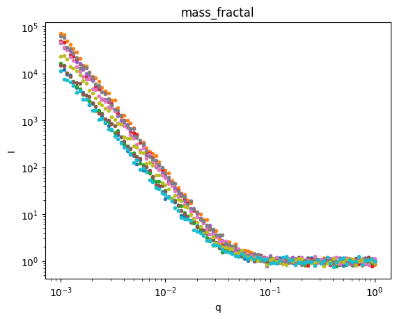
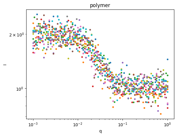

Excellent! It looks like we got a perfect separation, even between the two fractal models.
Conclusion#
In this example, we demonstrated a complete workflow for fitting multiple SAS models to data and automatically selecting the best model based on chi-squared values. While this example used simulated data that was specifically generated to be well-separated between different model types (making the fitting and model selection relatively straightforward), it illustrates the key components and capabilities of the AutoSAS pipeline:
Fitting multiple models to the same dataset
Comparing fit quality across models
Automatically selecting the best model for each sample
With real experimental data, the fitting and model selection process may be more challenging due to:
Noise and experimental uncertainties
Samples that could be described by multiple models
More complex scattering patterns requiring more sophisticated models
However, the workflow demonstrated here provides a foundation for approaching these more complex cases in a systematic way.