![]()
Build an xarray.Dataset from Scratch#
In this How-To we’ll go through the process of building up an xarray.Dataset that could be used as an input to Pipeline.calculate. We’ll generate random compositions and fake data to go along with these compositions.
The dataset generated in this notebook is the basis for the Building Pipelines tutorial.
Google Colab Setup#
Only uncomment and run the next cell if you are running this notebook in Google Colab or if don’t already have the AFL-agent package installed.
[ ]:
# !pip install git+https://github.com/usnistgov/AFL-agent.git
First Steps#
To begin, let’s import the necessary libraries for this document and then make an empty :py:class:xarray.Dataset
[1]:
import numpy as np
import numpy as np
import xarray as xr
import matplotlib.pyplot as plt

ds = xr.Dataset()
ds
[1]:
<xarray.Dataset> Size: 0B
Dimensions:  ()
Data variables:
*empty*Compositions#
Next, we generate random ‘compositions’ that we’ll do simulated/virtual measurements at. We’ll generate the compositions for a 2-dimensional space with components “A” and “B” as placeholders. You could imagine that A and B are the concentrations of two different preservatives in a liquid mixtures.
[2]:
num_measurements = 100
A = np.random.uniform(0,10,size=num_measurements)
B = np.random.uniform(0,25,size=num_measurements)
compositions = np.array([A,B]).T
compositions
[2]:
array([[ 1.93506959,  4.33877746],
       [ 3.99993228, 15.11981127],
       [ 5.14403166,  1.65850983],
       [ 4.57883235, 12.34183192],
       [ 8.05567528, 10.47358865],
       [ 1.04161007, 22.83361697],
       [ 5.85757901, 18.81270953],
       [ 4.29558185, 16.91442648],
       [ 3.14950211,  2.08947439],
       [ 7.65251749, 13.05015789],
       [ 5.58833051,  7.55301393],
       [ 8.75864958, 13.90004698],
       [ 9.03579843,  1.04110731],
       [ 6.94709288, 22.03909555],
       [ 6.30872735, 23.08178649],
       [ 8.38214203, 24.28281802],
       [ 6.09861924,  5.67560421],
       [ 0.12177663,  1.50263558],
       [ 5.4271795 , 24.05339109],
       [ 3.32773495, 12.91733508],
       [ 8.22656778, 18.12750637],
       [ 7.77255352,  1.61982803],
       [ 1.58024907,  8.89957219],
       [ 0.62964449, 13.64241493],
       [ 4.87628903, 11.61657773],
       [ 5.13234999, 15.35880089],
       [ 3.02453785, 10.78092744],
       [ 6.29667967,  9.70296135],
       [ 2.87889006, 21.23149213],
       [ 7.33476093, 23.21218938],
       [ 6.96178175, 14.54078124],
       [ 9.94068744, 13.1306839 ],
       [ 5.81347609, 18.31807371],
       [ 3.65653358,  1.86819243],
       [ 8.97030945, 15.30596251],
       [ 2.93130382, 20.47763125],
       [ 9.37753719, 17.91516725],
       [ 0.41716654,  1.43289172],
       [ 1.1435741 ,  4.91629814],
       [ 1.08112256, 11.13119176],
       [ 5.25354877,  9.45231719],
       [ 7.20589227, 18.57879028],
       [ 7.89243271, 11.31509607],
       [ 6.94687163, 14.82218341],
       [ 7.23403931,  6.79257162],
       [ 8.68249381, 12.53839805],
       [ 1.06877839, 10.32097668],
       [ 7.89831494,  0.4644321 ],
       [ 1.55458517, 24.16727467],
       [ 0.45829217,  3.24497194],
       [ 8.9361479 , 15.47144486],
       [ 6.41770086, 10.88253153],
       [ 5.88298706, 18.25514364],
       [ 1.345648  , 11.08596411],
       [ 1.03642353, 21.48281264],
       [ 8.17349873, 17.80265345],
       [ 8.24719952, 23.52786849],
       [ 7.19131724,  9.11486603],
       [ 0.78123421,  3.94805308],
       [ 6.24072184, 17.0863877 ],
       [ 0.50409961, 16.27277289],
       [ 8.38188047,  1.72138619],
       [ 2.60295083,  4.67442285],
       [ 2.58444436, 16.57143555],
       [ 9.35239534, 16.00199993],
       [ 6.50574801, 17.33916381],
       [ 3.27476499,  7.83797279],
       [ 7.75461602, 23.60987228],
       [ 0.55448762, 24.08902153],
       [ 3.82063523, 20.43360895],
       [ 1.96279418,  8.66791611],
       [ 8.31501072,  0.0249756 ],
       [ 2.4606    ,  5.38843633],
       [ 9.1328654 , 19.8844552 ],
       [ 4.08471932,  1.10690158],
       [ 8.48469695, 11.10944636],
       [ 5.99946032, 10.58338866],
       [ 7.99427379, 10.09969   ],
       [ 8.71171219,  7.02035713],
       [ 7.30678607, 24.33877297],
       [ 7.76378269, 21.99343589],
       [ 7.45991402,  8.11174006],
       [ 7.63854343, 13.54025074],
       [ 0.81733253,  9.43775453],
       [ 7.20059135,  5.85811728],
       [ 2.20804772,  6.7721729 ],
       [ 3.65472461,  4.43961665],
       [ 8.21345636, 10.74735116],
       [ 9.92147334, 15.55468087],
       [ 9.52663079,  6.77762994],
       [ 7.01379838, 22.20232276],
       [ 0.23914684,  3.4963898 ],
       [ 3.46456904, 12.84968187],
       [ 0.26618359,  8.12557401],
       [ 1.1156883 ,  0.45431966],
       [ 6.91416382, 21.4816626 ],
       [ 0.59623227,  7.69198605],
       [ 2.02031934,  4.93580074],
       [ 5.21402634,  4.84272796],
       [ 7.87824238, 14.33035062]])
Now let’s add this information to the :py:class:xarray.Dataset.
Note how, for the composition variable, we need to not only specify the name of the variable in the dataset but also the names of the dimensions of the data (‘sample’ and ‘components’).
[3]:
ds['composition'] = (['sample','component'],compositions)
ds['component'] = ('component',['A','B'])
ds
[3]:
<xarray.Dataset> Size: 2kB
Dimensions:      (sample: 100, component: 2)
Coordinates:
  * component    (component) <U1 8B 'A' 'B'
Dimensions without coordinates: sample
Data variables: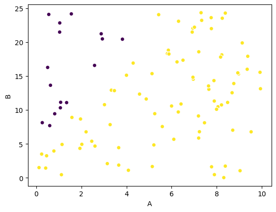
composition (sample, component) float64 2kB 1.935 4.339 4.0 ... 7.878 14.33Okay, in order to simulate a ‘phase boundary’ we’ll create labels for the data. We’ll draw an arbitrary line through the composition space and label the data that is above and below that line.
Let’s generate this data and add it to the dataset
[4]:
labels = (A>(0.25*B-1)).astype(int)
ds['ground_truth_labels'] = ('sample',labels)
ds
[4]:
<xarray.Dataset> Size: 2kB
Dimensions:              (sample: 100, component: 2)
Coordinates:
  * component            (component) <U1 8B 'A' 'B'
Dimensions without coordinates: sample
Data variables:
    composition          (sample, component) float64 2kB 1.935 4.339 ... 14.33
ground_truth_labels (sample) int64 800B 1 1 1 1 1 0 1 1 ... 1 0 1 1 0 1 1 1Now we can plot the data. We do this using xarray by first extracting the compositions data variable into a new standalone xarray.Dataset and then calling plot.scatter on it.
[5]:
ds.composition.to_dataset('component').plot.scatter(x='A',y='B',c=ds.ground_truth_labels)
plt.show()
Simulated Measurement Data#
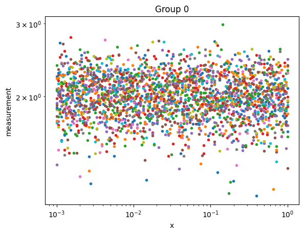
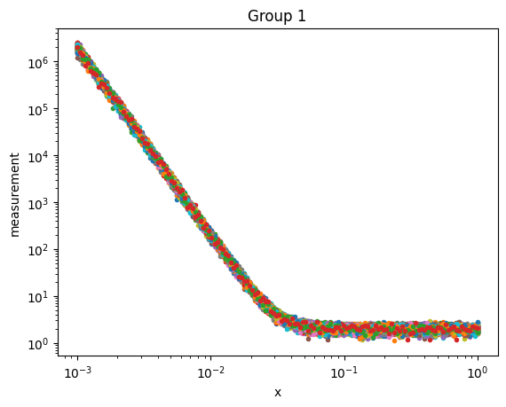
Now let’s generate the ‘measurement’ data. We’ll generate one measurement for each composition generated above. We’ll generate two kinds of data that depend on the data label:
A flat background signal with random Gaussian noise
A power-law with a power of -4 that decays to a flat background
Both kinds of data will have random Gaussian noise.
Now we can define a method (Python’s name for a function) that randomly generates one of two measurement signals.
[6]:
import numpy as np

def measure(x,label):
    """Generate one of two signals with noise"""

    if label==0:
        m = np.ones_like(x) #flat background
    else:
        m = 1e-6*np.power(x,-4) + 1.0  #power law

    # add noise
    m += np.random.normal(loc=m, scale=0.25*m, size=x.shape[0])

    return m
Let’s define a domain for the measurement (x), generate the data, and the create an xarray.Dataset with it.
[7]:
import xarray as xr

#domain of the measurements (e.g., for scattering this would be q, for
#spectroscopy this would be wavelength or wavenumber)
x = np.geomspace(0.001,1.0,150)

# conduct 50 measurements and gather into an array
measurements = np.array([measure(x,label) for label in labels])

# add the measurement data to the dataset
ds['measurement'] = (['sample','x'],measurements)
ds['ground_truth_labels'] = (['sample'],labels)
ds['x'] = ('x',x)
ds
[7]:
<xarray.Dataset> Size: 124kB
Dimensions:              (sample: 100, component: 2, x: 150)
Coordinates:
  * component            (component) <U1 8B 'A' 'B'
  * x                    (x) float64 1kB 0.001 0.001047 0.001097 ... 0.9547 1.0
Dimensions without coordinates: sample
Data variables:
    composition          (sample, component) float64 2kB 1.935 4.339 ... 14.33
    ground_truth_labels  (sample) int64 800B 1 1 1 1 1 0 1 1 ... 1 0 1 1 0 1 1 1
measurement (sample, x) float64 120kB 2.047e+06 1.318e+06 ... 2.065Now let’s plot the two groups of data
[8]:
for label, sub_ds in ds.groupby('ground_truth_labels'):
    plt.figure()
    sub_ds.measurement.plot.line(x='x',marker='.',ls='None',xscale='log',yscale='log',add_legend=False)
    plt.title(f'Group {label}')

plt.show()
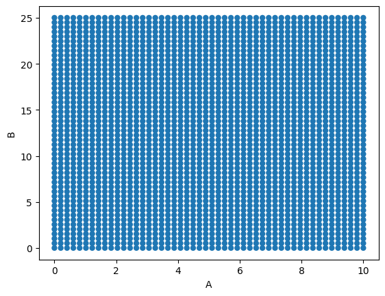
Composition Grid#
Okay, the final piece of data that you need to start is the composition grid. This grid defines the space that the agent will evaluate when choosing the next composition
[9]:
num_grid_points = 50
A_grid = np.linspace(0,10,num_grid_points)
B_grid = np.linspace(0,25,num_grid_points)
composition_grid = np.meshgrid(A_grid,B_grid)
composition_grid = np.array([composition_grid[0].ravel(),composition_grid[1].ravel()]).T

ds['composition_grid'] = (['grid','component'],composition_grid)
ds
[9]:
<xarray.Dataset> Size: 164kB
Dimensions:              (sample: 100, component: 2, x: 150, grid: 2500)
Coordinates:
  * component            (component) <U1 8B 'A' 'B'
  * x                    (x) float64 1kB 0.001 0.001047 0.001097 ... 0.9547 1.0
Dimensions without coordinates: sample, grid
Data variables:
    composition          (sample, component) float64 2kB 1.935 4.339 ... 14.33
    ground_truth_labels  (sample) int64 800B 1 1 1 1 1 0 1 1 ... 1 0 1 1 0 1 1 1
    measurement          (sample, x) float64 120kB 2.047e+06 1.318e+06 ... 2.065
composition_grid (grid, component) float64 40kB 0.0 0.0 ... 10.0 25.0Let’s inspect the grid in a plot
[10]:
ds.composition_grid.to_dataset('component').plot.scatter(x='A',y='B',edgecolor='None')
plt.show()
Saving the Dataset to disk#
We can save this dataset to disk for use in other notebooks or to memorialize the input data used in a calculation. We’ll use the netcdf format for this:
[11]:
ds.to_netcdf('../data/example_dataset.nc')
Conclusion#
In this notebook, we demonstrated how to build an xarray.Dataset from scratch.
We:
Created an empty dataset
Added composition data for samples
Added ground truth labels for the samples
Added simulated measurement data
Added a composition grid for the agent to explore
Saved the dataset to disk in netCDF format
The resulting dataset contains all the necessary components for training and evaluating an active learning agent:
Sample compositions and their corresponding measurements
Ground truth labels for validation
A grid defining the composition space for exploration
This dataset structure represents a typical format expected by many agent pipelines in AFL.double_agent. The exact variables and variable names will change with the pipeline, but the concept of having measurement data and composition information that shares dimensions is a foundational feature of analyzing formulations and materials problems where the composition is varying.